Testing approaches under non-proportional hazards using R

Introduction

In clinical studies with time-to-event outcomes, it is commonly assumed that the hazard functions of two groups are proportional. The standard log-rank test is widely used to test the equivalence of survival functions. It assumes no relationship between the censoring indicator and the forecast, such that dropouts or individuals who are not fully observed are perceived to be the same in risks (sensitivity to proportional risk); the events are also weighted equally regardless of time of occurrence ( early/ late). However, several scenarios can lead to non-proportional hazards (NPH). For example, a delayed treatment effect may be observed in the treatment arm, which can lead to a departure from proportionality of the survival curves. Log-rank test loses power under the non-proportional hazard assumption. Thus, there are many tests available in the literature that can handle such scenarios. Most commonly used tests are as follows:

Weighted log-rank test.
Restricted Mean Survival Time (RMST).
Milestone survival.
Max-Combo test.
Modestly Weighted log-rank test.

This particular document focuses mainly on the weighted log-rank test, Max-combo test and Modestly Weighted log-rank. Some of the functions include:

wlrt()

This function uses $G(\rho,\gamma)=\hat{S}(t)^\rho (1-\hat{S}(t))^\gamma; \rho,\gamma \geq 0$ , where $\hat{S}(t)$ is the Kaplan-Meier estimate of the survival function at time $t$. If $\rho = \gamma = 0$, then this is the standard log-rank test. When $\rho=1, \gamma=0$ this test can be used to detect early difference in the survival curves; when $\rho=0, \gamma = 1$, this test can be used to detect late differences in the survival curves and when $\rho=1, \gamma = 1$, this test can be used to test middle differences in the survival curves. This is enabled by specifying method=fh in R as illustrated in the Peto-Peto Prentice test below. Also it is to be noted that this test gives the Z-score as the test statistic which can be squared to obtain the chi-square statistic. The function also supports the log-rank test: Method=lr and Modestly Weighted Log-rank test: method=mw.

survdiff()

This function uses $G(\rho)=\hat{S}(t)^\rho, \rho \geq 0$ , where $\hat{S}(t)$ is the Kaplan-Meier estimate of the survival function at time $t$. If $\rho = 0$, then this is the standard log-rank test.

Data.

Data source: https://stats.idre.ucla.edu/sas/seminars/sas-survival/

The data include 500 subjects from the Worcester Heart WHAS Study (WHAS500). This study examined several factors, such as age, gender and BMI, that may influence survival time after a heart WHAS. Follow-up time for all participants begins at the time of hospital admission after the WHAS and ends with death or loss to follow-up (censoring). The data in the WHAS500 are subject to right-censoring only. The variables used here are:

lenfol: length of follow-up, terminated either by death or censoring - time variable
fstat: loss to followup = 0, death = 1 - censoring variable
afb: atrial fibrillation, no = 0, 1 = yes - covariate
gender: males = 0, females = 1 - stratification factor

library(haven)
knitr::opts_chunk$set(echo = TRUE)
library(here)
WHAS <- haven::read_sas("../data/whas500.sas7bdat")
head(WHAS)

# A tibble: 6 × 19
     ID   AGE GENDER    HR SYSBP DIASBP   BMI   CVD   AFB   SHO   CHF   AV3
  <dbl> <dbl>  <dbl> <dbl> <dbl>  <dbl> <dbl> <dbl> <dbl> <dbl> <dbl> <dbl>
1     1    83      0    89   152     78  25.5     1     1     0     0     0
2     2    49      0    84   120     60  24.0     1     0     0     0     0
3     3    70      1    83   147     88  22.1     0     0     0     0     0
4     4    70      0    65   123     76  26.6     1     0     0     1     0
5     5    70      0    63   135     85  24.4     1     0     0     0     0
6     6    70      0    76    83     54  23.2     1     0     0     0     1
# ℹ 7 more variables: MIORD <dbl>, MITYPE <dbl>, YEAR <dbl>, LOS <dbl>,
#   DSTAT <dbl>, LENFOL <dbl>, FSTAT <dbl>

Kaplan-Meier Survival Curve.

Below is the Kaplan-Meier survival curve. Let:

$S_1(t)$: survival function for individuals with no atrial fibrillation(AFB=0)
$S_2(t)$: survival function for individuals with no atrial fibrillation(AFB=1)

Null hypothesis $H_0$: $S_1(t) = S_2(t)\quad \text{for all } t$

Alternative hypothesis $H_1$: $S_1(t) \neq S_2(t) \quad \text{for some } t$

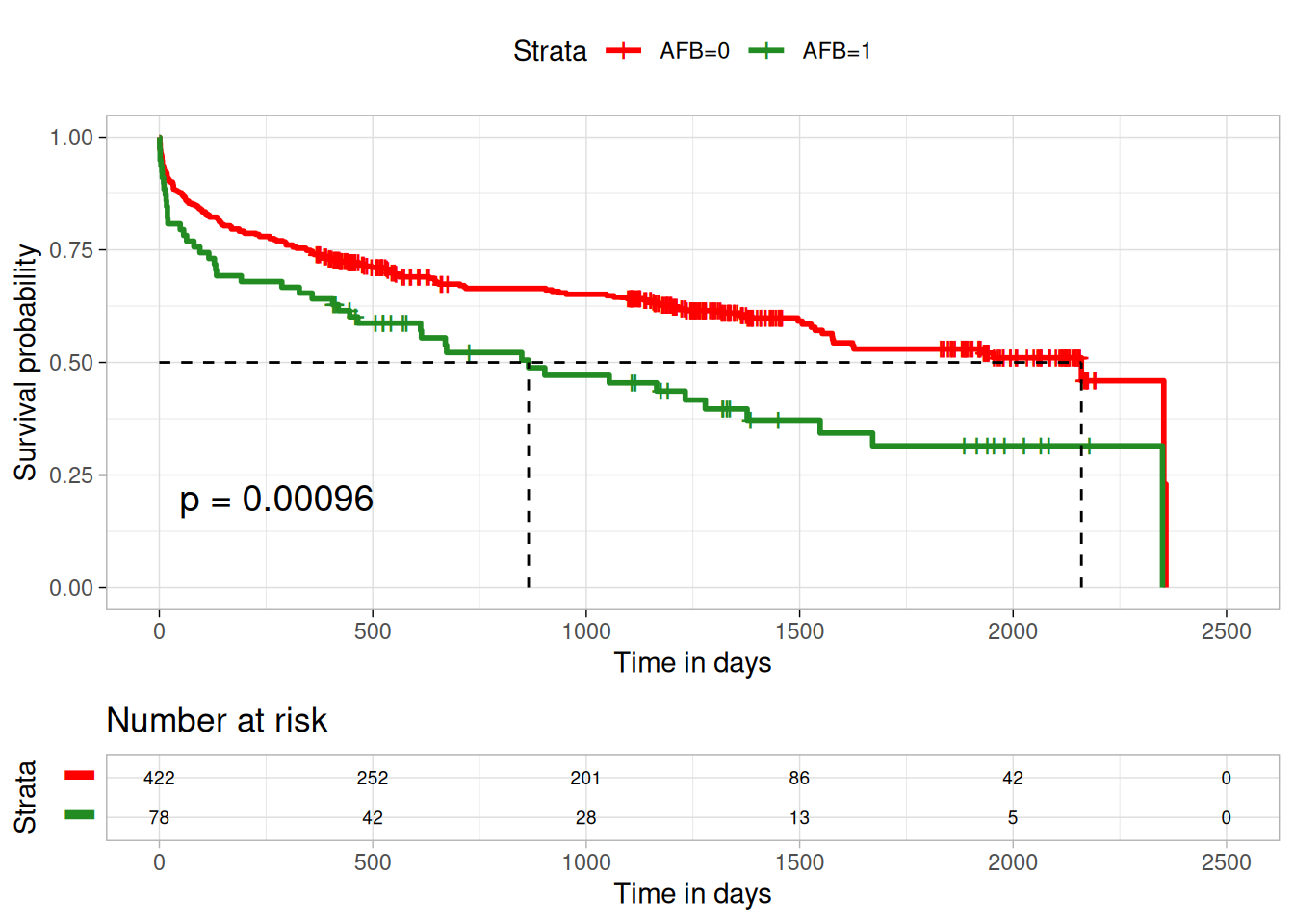
The p-value for the standard log-rank test is 0.00096. Since $0.00096< 0.05$, we reject the null hypothesis and conclude that there is statistically significant evidence that the survival distributions differ between the AFB groups over time. Individuals with no atrial fibrillation(AFB=0) have higher survival rates after a heart WHAS, compared to those with atrial fibrillation(AFB=1). Immediately after time 0, the curve for AFB=1 drops soon below the curve for AFB=0. This suggests that atrial fibrillation has a strong impact (early effect) on mortality after a heart WHAS.

library(survival) 
KM <- survfit(Surv(LENFOL, FSTAT)~AFB, data = WHAS)
ggsurvplot(KM,                     
   data = WHAS,            
   risk.table = TRUE, pval = TRUE, 
   palette = c("red","forestgreen"),
   conf.int = FALSE,         
   xlim = c(0,2500),         
   xlab = "Time in days",   
   break.time.by = 500,     
   ggtheme = theme_light(), 
 risk.table.y.text.col = T, 
  risk.table.y.text = FALSE,
 risk.table.fontsize=2.5,
 surv.median.line = "hv"
)

Warning: Using `size` aesthetic for lines was deprecated in ggplot2 3.4.0.
ℹ Please use `linewidth` instead.
ℹ The deprecated feature was likely used in the ggpubr package.
  Please report the issue at <https://github.com/kassambara/ggpubr/issues>.

Ignoring unknown labels:
• colour : "Strata"

Tests:

1. Weighted Log-Rank test.

The Weighted log-rank has been utilised in studies with non-proportional hazards to maximise power. By pre-specifying the weights, type I error is preserved. The choice of weight can be based on initial information or anticipated study design.
Suppose we have two groups (e.g. treatment and control, male and female, etc.) with survival functions $S_1$ and $S_2$, respectively. The null and alternative hypotheses are given as: \[H_0 : S_1(t)=S_2(t) \mbox{ }\forall t \mbox{ v/s } H_1 : S_1(t) \neq S_2(t) \mbox{ for some t. }\] Since the alternative hypothesis is composite, it includes multiple scenarios. Hence, the power calculation is difficult to implement. One way to tackle this situation is to consider the Lehman alternative given by $H_L : S_1(t)=(S_2(t))^\psi$ for all $t$ where $0<\psi<1$. Alternatively, \[ H_0 : \psi=1 \ v/s \ H_1: \psi<1\]

which implies subjects in group 1 will have longer survival times than subjects in group 2. For more details, refer to Page 44 of Moore (2016).
The test statistic for the weighted log-rank test is given by, \[ Z = \frac{\sum_{j=1}^{D}w_j(o_{j} -e_j)}{\sqrt{\sum_{j=1}^{D}w_j^2 v_j}} \to N(0,1), \text{under} \ H_0\] Equivalently, \[ Z^2 = \frac{\big[\sum_{j=1}^{D}w_j(o_j -e_j)\big]^2}{\sum_{j=1}^{D}w_j^2 v_j} \to \chi^2_1, \text{under} \ H_0.\]
Here, $t_1<t_2<...<t_D$ be the distinct failure time points of both the groups together. $o_j$ is the number of deaths, $e_j$ is the expected number of deaths, and $v_j$ is the variance of the number of deaths in either of the two groups.
Different weight functions are discussed in the literature, and a family of weight functions $G(\rho)$ is proposed by Harrington and Fleming (1982), which is implemented in R using survival : : survdiff (). Further, Fleming and Harrington (1991) extended the $G(\rho)$ family to $G(\rho,\gamma)$, and it is implemented in R using nphRCT : : wlrt().
Suppose $W_k$ is a positive weight function,$n_k$ is the size of the risk set, and $S(t_k)$ is the survival function. We can implement these tests by assigning different weights, such that:

- $W _k$= 1 [Weight=1] $\implies$ Log-rank test.
- $W_k$= $n_k$ [weights by risk set size] $\implies$ Wilcoxon test.
- $W_k$= $(n_k)^{1/2}$ [square root of risk set size] $\implies$ Tarone-Ware test.
- $W_k$= $(S(t_k))$ [weights by pooled survival function] $\implies$ Peto-Peto test.
- $W_k$= $(S(t_k))\frac{n_k}{n_k+1}$ [survival weight adjusted by risk set size] $\implies$ Modified Peto-Peto test.
- $W_k$= $\{S(t_k)\}^{\rho}\{1 - S(t_k)\}^{\gamma}$ [flexible survival-based weighting] $\implies$ Fleming-Harrington($\rho,\gamma$) test.

a). Peto-Peto

This test assigns weights based on the pooled Kaplan–Meier survival estimate$(S(t_k))$. Larger weights are assigned to earlier failures, thereby enabling greater emphasis on group differences at earlier times. This test can be implemented in R using these functions:

i) `survminer::surv_pvalue()`

The survminer::surv_pvalue() function calculates the p-value for comparing survival curves, while surv_fit() estimates the survival probabilities for groups defined by AFB. Using surv_pvalue(method = "S1") applies the Peto–Peto test via the survMisc package to assess group differences. The survMisc package (version 0.5.6) provides a collection of functions for analysing right-censored survival data, extending the methods available in the survival package. In particular, the comp function can be used to compare survival curves and print the corresponding p-value. Note that survMisc was archived on March 17, 2026, and is no longer available on CRAN.

fit <- surv_fit(Surv(LENFOL, FSTAT)~AFB, data = WHAS)
surv_pvalue(fit,
            method = "S1")

  variable   pval    method   pval.txt
1      AFB 0.0017 Peto-Peto p = 0.0017

# Extending the decimal places for the p-value
p<-surv_pvalue(fit, method="S1")$pval
sprintf("%.9f", p)

[1] "0.001700000"

The code below generates the test statistics for Peto-Peto using custom R function. The implementation is based on a classical statistical definition without reliance on external packages. survminer::surv_pvalue() rounds off the p-value to 4 decimal places internally. This is why extending the p-value manually yields zeros beyond the 4 decimal places. Rounding off the custom R p-values to 4 decimal places, generates p-values similar to those from survminer::surv_pvalue() . The custom R function also generates the chi-square test statistic, which is not enabled by the survminer package.

peto_peto_test <- function(formula, data) {
  mf <- stats::model.frame(formula, data)
  surv <- mf[[1]]
  time <- surv[, "time"]
  status <- ifelse(surv[, "status"] == 2, 1, surv[, "status"])
  group <- as.factor(mf[[2]])
  groups <- levels(group)
  event_times <- sort(unique(time[status == 1]))
  k <- length(event_times)   # number of event times
  g <- length(groups)        # number of groups
  # Risk set and event count matrices
  n_jk <- d_jk <- matrix(0, k, g)
  for (j in seq_len(g)) {
    t_j <- time[group == groups[j]]
    s_j <- status[group == groups[j]]
    for (i in seq_len(k)) {
      ti <- event_times[i]
      n_jk[i, j] <- sum(t_j >= ti)
      d_jk[i, j] <- sum(t_j == ti & s_j == 1)
    }
  }
  # Totals
  n_i <- rowSums(n_jk)
  d_i <- rowSums(d_jk)
  w <- cumprod(1 - d_i / (n_i + 1)) # ---- Peto-Peto weights (S1) ----
  # ---- 2-group test ----
  e1 <- n_jk[, 1] * d_i / n_i
  Q <- sum(w * (d_jk[, 1] - e1))
  VarQ <- sum(
    w^2 * n_jk[, 1] * n_jk[, 2] * d_i * (n_i - d_i) /
      (n_i^2 * (n_i - 1)),
    na.rm = TRUE
  )
  chisq <- (Q^2) / VarQ
  pvalue <- stats::pchisq(chisq, df = 1, lower.tail = FALSE)
  list(
    chisq = chisq,
    df = 1,
    pvalue = pvalue,
    method = "Peto-Peto (S1)"
  )
}
peto_peto_test(Surv(LENFOL, FSTAT)~AFB, data = WHAS)

$chisq
[1] 9.823786

$df
[1] 1

$pvalue
[1] 0.001722693

$method
[1] "Peto-Peto (S1)"

ii) `coin::logrank_test()`

coin package implements a conditional inference framework based on permutation tests. The log-rank test is one of the conditional test procedures that provides the weighted log-rank test reformulated as a linear rank test. The p-value is obtained from the conditional null distribution of the test statistic, and the asymptotic approximation of the exact distribution is used by default (distribution="Asymptotic"). The distribution can also be approximated via Monte Carlo resampling or computed exactly for the univariate two-sample problem by specifying the distribution as approximate or exact, respectively.

#Asymptotic
WHAS$AFB <- as.factor(WHAS$AFB)
logrank_test(Surv(WHAS$LENFOL, WHAS$FSTAT) ~ AFB, data = WHAS,
             type = "Peto-Peto",
             distribution = "asymptotic")


    Asymptotic Two-Sample Peto-Peto Test

data:  Surv(WHAS$LENFOL, WHAS$FSTAT) by AFB (0, 1)
Z = 3.0423, p-value = 0.002348
alternative hypothesis: true theta is not equal to 1

For exact distribution, computing exact permutation distribution was computationally intensive in this case and demanded large memory, hence returned an error. This can be due to many events as well as large sample size, which makes the computation combinatorialy intensive.

#Exact
#logrank_test(Surv(LENFOL,FSTAT) ~ AFB, data = WHAS,
            #type = "Peto-Peto",
           #distribution = "exact")

approximate distribution uses Monte Carlo re-sampling to approximate the distribution.

#Approximate
logrank_test(Surv(LENFOL,FSTAT)~AFB, data = WHAS,
             type = "Peto-Peto",
             distribution = "approximate")


    Approximative Two-Sample Peto-Peto Test

data:  Surv(LENFOL, FSTAT) by AFB (0, 1)
Z = 3.0423, p-value = 0.0029
alternative hypothesis: true theta is not equal to 1

iii) `survival::survdiff()`

survival::survdiff() tests if there is a difference between two or more survival curves using the $G^\rho$ family of tests, or for a single curve against a known alternative and with $\rho$=1, it is equivalent to the Peto & Peto modification of the Gehan-Wilcoxon test. The p-value generated is 0.0016528 . survminer::surv_pvalue() generates a p-value of 0.0017 for the same test. This subtle difference can be caused by the fact that these two functions: survival::survdiff(rho = 1) implements the $G^\rho$ test with weights $S(t)^\rho$, whereas survminer:: surv_pvalue() test uses weight of a modified pooled survival estimate S1. Mathematically, these methods can be represented as:

Assume : $t_i$ for $i=1,…,T$ are possible event times, $n_{ti}$is the overall risk set size on the time$t_i$, $e_{ti}$number of overall expected events in the time$t_i$ and $w{t_i}$ is a weight for the statistic, then S1Peto-Peto’s modified survival estimate: \[ w(t_i) = \hat{S}_1(t_i) = \prod_{t_i = 1}^{T} \left(1 - \frac{e_{t_i}}{n_{t_i} + 1} \right) \]

The survdiff function uses $G(\rho)=\hat{S}(t_i)^\rho, \rho \geq 0$ , where $\hat{S}(t_i)$ is the Kaplan-Meier estimate of the survival function at time $t_i$.

\[ \hat{S}_1(t_i) = \prod_{t_i = 1}^{T} \left(1 - \frac{e_{t_i}}{n_{t_i}} \right) \]

(L<- survival::survdiff(
  survival::Surv(LENFOL, FSTAT)~AFB,rho = 1,data = WHAS))

Call:
survival::survdiff(formula = survival::Surv(LENFOL, FSTAT) ~ 
    AFB, data = WHAS, rho = 1)

        N Observed Expected (O-E)^2/E (O-E)^2/V
AFB=0 422    130.1    142.8      1.14       9.9
AFB=1  78     36.4     23.7      6.84       9.9

 Chisq= 9.9  on 1 degrees of freedom, p= 0.002

# Extending the decimal places for p-value
chisq_value<-L$chisq
p_value<-1-pchisq(chisq_value, df = length(L$n) - 1)
cat("p-value=", format(p_value,digits = 9), "\n")

p-value= 0.00165276596

b). Modified Peto-Peto.

i). `survminer::surv_pvalue()`

fit.null <- surv_fit(Surv(LENFOL,FSTAT)~AFB, data = WHAS)
surv_pvalue(fit.null,
            method = "S2")

  variable   pval             method   pval.txt
1      AFB 0.0018 modified Peto-Peto p = 0.0018

# Extending the decimal places for the p-value
p<-surv_pvalue(fit, method="S2")$pval
sprintf("%.9f", p)

[1] "0.001800000"

Just like for Peto-Peto, the code below generates the test statistics for Modified Peto-Peto using custom R function.

modified_peto_peto_test <- function(formula, data) {
  mf <- stats::model.frame(formula, data)
  surv <- mf[[1]]
  time <- surv[, "time"]
  status <- ifelse(surv[, "status"] == 2, 1, surv[, "status"])
  group <- as.factor(mf[[2]])
  groups <- levels(group)
  event_times <- sort(unique(time[status == 1]))
  k <- length(event_times)   # number of event times
  g <- length(groups)        # number of groups
  # Risk set and event count matrices
  n_jk <- d_jk <- matrix(0, k, g)
  for (j in seq_len(g)) {
    t_j <- time[group == groups[j]]
    s_j <- status[group == groups[j]]
    for (i in seq_len(k)) {
      ti <- event_times[i]
      n_jk[i, j] <- sum(t_j >= ti)
      d_jk[i, j] <- sum(t_j == ti & s_j == 1)
    }
  }
  # Totals
  n_i <- rowSums(n_jk)
  d_i <- rowSums(d_jk)
  s1 <- cumprod(1 - d_i / (n_i + 1))# ---- Modified Peto-Peto weights (S2) ----
  w  <- s1 * n_i / (n_i + 1)
  # ---- 2-group test ----
  e1 <- n_jk[, 1] * d_i / n_i
  Q <- sum(w * (d_jk[, 1] - e1))
  VarQ <- sum(
    w^2 * n_jk[, 1] * n_jk[, 2] * d_i * (n_i - d_i) /
      (n_i^2 * (n_i - 1)),
    na.rm = TRUE
  )
  chisq <- (Q^2) / VarQ
  pvalue <- stats::pchisq(chisq, df = 1, lower.tail = FALSE)
  list(chisq = chisq,df = 1,pvalue = pvalue,method = "Modified Peto-Peto (S2)"
  )
}
modified_peto_peto_test(Surv(LENFOL, FSTAT)~AFB, data = WHAS)

$chisq
[1] 9.749083

$df
[1] 1

$pvalue
[1] 0.001794122

$method
[1] "Modified Peto-Peto (S2)"

ii). `coin::logrank_test()`

logrank_test(Surv(LENFOL, FSTAT)~AFB,data = WHAS,type = "Andersen-Borgan-Gill-Keiding",
distribution = "asymptotic"
)


    Asymptotic Two-Sample Andersen-Borgan-Gill-Keiding Test

data:  Surv(LENFOL, FSTAT) by AFB (0, 1)
Z = 3.0276, p-value = 0.002465
alternative hypothesis: true theta is not equal to 1

c). Tarone-Ware.

i). `survminer::surv_pvalue()`

It balances sensitivity between early and late differences. The survdiff() function implements the $G(\rho)$ family with parameter $\rho$ but does not include the Tarone-Ware option; Tarone-Ware weight is proportional to $\sqrt{n_k}$, which is not of the $\hat{S}(t)^\rho$ family; therefore, it should not be implemented as rho= option. Therefore, in this function, there is no inbuilt implementation of Tarone-Ware option, although some analysts approximate it by suggesting $\rho$= 0.5, such that it assigns weights between standard log_rank ($\rho$= 0) and tests that emphasise on early events like Gehan-Breslow. For this document, computation is based on the definition of Tarone-Ware, which is weighted by taking the square root of the risk set $\sqrt{n_k}$. This is possible to define in the survminer package.

The survminer package enables R functions for visualisation and survival analysis. survminer::surv_pvalue() function enables one to specify the weight sqrtN for Tarone-Ware in R. This outputs only the p-value of the specified test. The package does not have an inbuilt function to generate the test statistic.

fit<-survfit(Surv(LENFOL, FSTAT)~AFB, data = WHAS)
surv_pvalue(fit,method="sqrtN")

  variable   pval      method   pval.txt
1      AFB 0.0022 Tarone-Ware p = 0.0022

# Extending the decimal places for the p-value
p<-surv_pvalue(fit, method="SqrtN")$pval
sprintf("%.9f", p)

[1] "0.002200000"

Just like for Peto-Peto, the code below generates the test statistics for the Tarone-Ware test based on this custom R function.

tarone_ware_test <- function(formula, data) {
  mf <- stats::model.frame(formula, data)
  surv <- mf[[1]]
  time <- surv[, "time"]
  status <- ifelse(surv[, "status"] == 2, 1, surv[, "status"])
  group <- as.factor(mf[[2]])
  groups <- levels(group)
  event_times <- sort(unique(time[status == 1]))
  k <- length(event_times)
  g <- length(groups)
  n_jk <- d_jk <- matrix(0, k, g)
  for (j in seq_len(g)) {
    t_j <- time[group == groups[j]]
    s_j <- status[group == groups[j]]
    for (i in seq_len(k)) {
      ti <- event_times[i]
      n_jk[i,j] <- sum(t_j >= ti)
      d_jk[i,j] <- sum(t_j == ti & s_j == 1)
    }
  }
  n_i <- rowSums(n_jk)
  d_i <- rowSums(d_jk)
  w <- sqrt(n_i)   # Tarone-Ware weight
  e1 <- n_jk[,1] * d_i / n_i
  Q <- sum(w * (d_jk[,1] - e1))
  VarQ <- sum(
    w^2 * n_jk[,1] * n_jk[,2] * d_i * (n_i - d_i) /
    (n_i^2 * (n_i - 1)),
    na.rm = TRUE
  )
  chisq <- (Q^2) / VarQ
  pvalue <- stats::pchisq(chisq, df = 1, lower.tail = FALSE)
  list(chisq = chisq, df = 1, pvalue = pvalue, method = "Tarone-Ware")
}
tarone_ware_test(Surv(LENFOL, FSTAT)~AFB, data = WHAS)

$chisq
[1] 9.42297

$df
[1] 1

$pvalue
[1] 0.002142842

$method
[1] "Tarone-Ware"

ii) `coin::logrank_test()`

logrank_test(Surv(LENFOL, FSTAT)~AFB,data = WHAS,type = "Tarone-Ware",
distribution = "asymptotic"
)


    Asymptotic Two-Sample Tarone-Ware Test

data:  Surv(LENFOL, FSTAT) by AFB (0, 1)
Z = 2.9636, p-value = 0.003041
alternative hypothesis: true theta is not equal to 1

d). Gehan-Breslow.

i). `survminer::surv_pvalue()`

The survdiff() function implements the $G(\rho)$ family with parameter $\rho$ but does not include Gehan-Breslow; Gehan-Breslow weight is proportional to $n_k$, which is not of the $\hat{S}(t)^\rho$ family; therefore, it is not implemented as rho= option. Therefore, there is no inbuilt implementation of the Gehan-Breslow option, although some analysts approximate it by suggesting $\rho$=1 such that it assigns weights by emphasising on early events. Here, we make a consideration based on the definition of Gehan-Breslow, which is weighted by taking the total risk set $n_k$. survminer::surv_pvalue() function enables one to specify the weight n for Gehan-Breslow in R. This outputs only the p-value of the specified test. The package does not have an inbuilt function to generate the test statistic.

fit<-survfit(Surv(LENFOL, FSTAT)~AFB, data = WHAS)
library(survminer)
surv_pvalue(fit,method="n")

  variable   pval        method   pval.txt
1      AFB 0.0041 Gehan-Breslow p = 0.0041

# Extending the decimal places for the p-value
p<-surv_pvalue(fit, method="n")$pval
sprintf("%.9f", p)

[1] "0.004100000"

The same custom R function is modified and implemented for the Gehan-Breslow Weighted Log-rank test. This procedure provides a similar p-value as that of survminer::surv_pvalue() but again outputs the test statistic, which is not enabled by survminer package.

Gehan_Breslow_test <- function(formula, data) {
  mf <- stats::model.frame(formula, data)
  surv <- mf[[1]]
  time <- surv[, "time"]
  status <- ifelse(surv[, "status"] == 2, 1, surv[, "status"])
  group <- as.factor(mf[[2]])
  groups <- levels(group)
  event_times <- sort(unique(time[status == 1]))
  k <- length(event_times)
  g <- length(groups)
  n_jk <- d_jk <- matrix(0, k, g)
  for (j in seq_len(g)) {
    t_j <- time[group == groups[j]]
    s_j <- status[group == groups[j]]
    for (i in seq_len(k)) {
      ti <- event_times[i]
      n_jk[i,j] <- sum(t_j >= ti)
      d_jk[i,j] <- sum(t_j == ti & s_j == 1)
    }
  }
  n_i <- rowSums(n_jk)
  d_i <- rowSums(d_jk)
  w <- n_i  # Gehan-Breslow weight
  e1 <- n_jk[,1] * d_i / n_i
  Q <- sum(w * (d_jk[,1] - e1))
  VarQ <- sum(
    w^2 * n_jk[,1] * n_jk[,2] * d_i * (n_i - d_i) /
    (n_i^2 * (n_i - 1)),
    na.rm = TRUE
  )
  chisq <- (Q^2) / VarQ
  pvalue <- stats::pchisq(chisq, df = 1, lower.tail = FALSE)
  list(chisq = chisq, df = 1, pvalue = pvalue, method = "Gehan-Breslow")
}
Gehan_Breslow_test(Surv(LENFOL, FSTAT)~AFB, data = WHAS)

$chisq
[1] 8.259274

$df
[1] 1

$pvalue
[1] 0.004054433

$method
[1] "Gehan-Breslow"

ii) `coin::logrank_test()`

logrank_test(Surv(LENFOL, FSTAT)~AFB,data = WHAS,type = "Gehan-Breslow",
distribution = "asymptotic"
)


    Asymptotic Two-Sample Gehan-Breslow Test

data:  Surv(LENFOL, FSTAT) by AFB (0, 1)
Z = 2.7863, p-value = 0.005331
alternative hypothesis: true theta is not equal to 1

e). Fleming-Harrington

i). `nphRCT::wlrt()`

This test is implemented using the function wlrt() from the nphRCT package. This function uses $G(\rho,\gamma)=\hat{S}(t)^\rho (1-\hat{S}(t))^\gamma; \rho,\gamma \geq 0$ (Fleming-Harrington test), where $\hat{S}(t)$ is the Kaplan-Meier estimate of the survival function at time $t$. When $\rho=1, \gamma=0$, this test can be used to detect early differences in the survival curves. To obtain the corresponding $p$-value, we can either use 2(1-pnorm(abs(ppp$z),0,1)) or we can square the test statistic WL$z by using (ppp$z)^2 and obtain the corresponding $p$-values as 1 - pchisq((ppp$z)^2,1); both the $p$-values will be the same.

#Places weight on hazards in the middle of the study.
(ppp <- nphRCT::wlrt(survival::Surv(LENFOL, FSTAT)~AFB,   
  data = WHAS,method = "fh",rho = 0.5,gamma = 0.5 ))

         u    v_u        z trt_group
1 6.312899 3.8646 3.211268         1

p<-2 * (1 - pnorm(abs(ppp$z), 0, 1))
cat("chisquare:", round(ppp$z^2, 4), "  p-value:", round(p, 4), "\n")

chisquare: 10.3122   p-value: 0.0013

#Places weight on hazards in the middle of the study.
(ppp <- nphRCT::wlrt(survival::Surv(LENFOL, FSTAT)~AFB,   
  data = WHAS,method = "fh",rho = 1,gamma = 1 ))

         u       v_u        z trt_group
1 2.669976 0.7272873 3.130793         1

p<-2 * (1 - pnorm(abs(ppp$z), 0, 1))
cat("chisquare:", round(ppp$z^2, 4), "  p-value:", round(p, 4), "\n")

chisquare: 9.8019   p-value: 0.0017

#Places weight on hazards at the end of the study.
(ppp <- nphRCT::wlrt(survival::Surv(LENFOL, FSTAT)~AFB,   
  data = WHAS,method = "fh",rho = 0,gamma = 1 ))

         u     v_u        z trt_group
1 4.042585 1.71206 3.089582         1

p<-2 * (1 - pnorm(abs(ppp$z), 0, 1))
cat("chisquare:", round(ppp$z^2, 4), "  p-value:", round(p, 4), "\n")

chisquare: 9.5455   p-value: 0.002

#Places weight on hazards at the end of the study.
(ppp <- nphRCT::wlrt(survival::Surv(LENFOL, FSTAT)~AFB,   
  data = WHAS,method = "fh",rho = 0.5,gamma = 2 ))

        u      v_u       z trt_group
1 1.07388 0.139906 2.87103         1

p<-2 * (1 - pnorm(abs(ppp$z), 0, 1))
cat("chisquare:", round(ppp$z^2, 4), "  p-value:", round(p, 4), "\n")

chisquare: 8.2428   p-value: 0.0041

#Places weight on hazards at the beginning of the study.
(ppp <- nphRCT::wlrt(survival::Surv(LENFOL, FSTAT)~AFB,   
  data = WHAS,method = "fh",rho = 1,gamma = 0 ))

         u      v_u       z trt_group
1 12.73229 16.37483 3.14643         1

p<-2 * (1 - pnorm(abs(ppp$z), 0, 1))
cat("chisquare:", round(ppp$z^2, 4), "  p-value:", round(p, 4), "\n")

chisquare: 9.9   p-value: 0.0017

ii). `coin::logrank_test()`

#Places weight on hazards in the middle of the study.
logrank_test(Surv(LENFOL, FSTAT)~AFB, data = WHAS,
             type = "Fleming-Harrington", rho = 0.5, gamma = 0.5,
             distribution = "asymptotic")


    Asymptotic Two-Sample Fleming-Harrington Test

data:  Surv(LENFOL, FSTAT) by AFB (0, 1)
Z = 3.0582, p-value = 0.002226
alternative hypothesis: true theta is not equal to 1

#Places weight on hazards in the middle of the study.
logrank_test(Surv(LENFOL, FSTAT)~AFB, data = WHAS,
             type = "Fleming-Harrington", rho = 1, gamma = 1,
             distribution = "asymptotic")


    Asymptotic Two-Sample Fleming-Harrington Test

data:  Surv(LENFOL, FSTAT) by AFB (0, 1)
Z = 2.972, p-value = 0.002958
alternative hypothesis: true theta is not equal to 1

#Places weight on hazards at the end of the study.
logrank_test(Surv(LENFOL, FSTAT)~AFB, data = WHAS,
             type = "Fleming-Harrington", rho = 0, gamma = 1,
             distribution = "asymptotic")


    Asymptotic Two-Sample Fleming-Harrington Test

data:  Surv(LENFOL, FSTAT) by AFB (0, 1)
Z = 2.9256, p-value = 0.003438
alternative hypothesis: true theta is not equal to 1

#Places weight on hazards at the end of the study.
logrank_test(Surv(LENFOL, FSTAT)~AFB, data = WHAS,
             type = "Fleming-Harrington", rho = 0.5, gamma = 2,
             distribution = "asymptotic")


    Asymptotic Two-Sample Fleming-Harrington Test

data:  Surv(LENFOL, FSTAT) by AFB (0, 1)
Z = 2.7163, p-value = 0.006601
alternative hypothesis: true theta is not equal to 1

  #Places weight on hazards at the beginning of the study.
logrank_test(Surv(LENFOL, FSTAT)~AFB, data = WHAS,
             type = "Fleming-Harrington", rho = 1, gamma = 0,
            distribution = "asymptotic")


    Asymptotic Two-Sample Fleming-Harrington Test

data:  Surv(LENFOL, FSTAT) by AFB (0, 1)
Z = 3.0423, p-value = 0.002348
alternative hypothesis: true theta is not equal to 1

Summary results for Weighted log-rank test.

Note: coin::logrank_test() - Default distribution is asymptotic. Generates $Z$ test statistic. $Z^2 = \chi^2_{(1)}$

Test	Function	Chi-square	P-Value
Peto - Peto	survminer: : surv_pvalue()	Null	0.0017
	custom R function	9.823786	0.001722693
	coin: : logrank_test()-asymptotic distribution	$Z$=3.0423 $Z^2$=9.2556	0.002348
	coin: : logrank_test()- approximate distribution	$Z$=3.0423 $Z^2$=9.2556	0.0022
	survival: : survdiff()	9.9	0.001652766
Modified Peto-Peto	survminer: : surv_pvalue()	Null	0.0018
	custom R function	9.749083	0.001794122
	coin: : logrank_test()	$Z$=3.0276 $Z^2$=9.1664	0.002465
Tarone-Ware	survminer: : surv_pvalue()	Null	0.00021
	custom R function	9.42297	0.002142842
	coin: : logrank_test()	$Z$= 2.9636 $Z^2$=8.7829	0.003041
Gehan- Breslow	survminer: : surv_pvalue()	Null	0.0041
	custom R function	8.259274	0.004054433
	coin: : logrank_test()	$Z$=2.7863 $Z^2$=7.7635	0.005331
Fleming-Harrington	nphRCT: : wlrt()
	FH(0.5, 0.5)	10.3122	0.0013
	FH(1, 1)	9.8019	0.0017
	FH(0, 1)	9.5455	0.002
	FH(0.5, 2)	8.2428	0.0041
	FH(1,0	9.9	0.0017
	coin: : logrank_test()
	FH(0.5, 0.5)	$Z$=3.0582 $Z^2$=9.3526	0.002226
	FH(1, 1)	$Z$=2.972 $Z^2$=8.8327	0.002958
	FH(0, 1)	$Z$=2.9256 $Z^2$=8.5591	0.0034938
	FH(0.5, 2)	$Z$=2.7163 $Z^2$=7.3783	0.006601
	FH(1, 0)	$Z$=3.0423 $Z^2$=9.2556	0.002348

2. Max-Combo test.

i). Max-Combo(No strata)

This is a universal criterion for examining the proximity of the survival functions, especially when no initial information about the trial is available. It combines multiple weighted log-rank criteria to enable sensitivity for equally, early, middle and late differences concurrently, such that it defines the maximum of the $G^{0,1}$ and $G^{1,0}$ criteria. It is also suitable when there is a violation of the proportional hazard assumption and uncertainty about the distribution of survival time.
The combination test aims for strong power to realise the survival curves difference over a range of possible alternative hypotheses. R software performs the combination test with an option to assign any set of weights using the function logrank.maxtest() from the nph package for comparison of two groups. logrank.maxtest() defaults to a two‑sided hypothesis, especially when no choice is made between the three in the alternative argument: alternative=c("two.sided", "less", "greater"). For this case, we specified to "two.sided". mvtnorm::GenzBretz() calls the Genz–Bretz algorithm, a quasi-Monte Carlo method, which introduces randomness in each run; this generates slightly varying values for the unadjusted p-value in each run. Therefore, there is a need to use set.seed() for reproducibility. Max-Combo two-sided statistic is defined as $Z_{\max} = \max(|Z_1|, |Z_2|, \ldots, |Z_k|)$. Therefore $Z_{\max}$= 3.30, and the two-sided unadjusted p-value is: 0.00196$\approx$ 0.002. Bonferroni corrected p-value is 0.00385.

set.seed(254)
logrank.maxtest(
  time   = WHAS$LENFOL,
  event  = WHAS$FSTAT,
  group  = WHAS$AFB,
  alternative = c("two.sided"),
  rho = c(0, 1, 0,1),
  gamma = c(0, 0, 1, 1),
  event_time_weights = NULL,
  algorithm = mvtnorm::GenzBretz(maxpts = 50000, abseps = 1e-05, releps = 0)
)

Call:
logrank.maxtest(time = WHAS$LENFOL, event = WHAS$FSTAT, group = WHAS$AFB, 
    alternative = c("two.sided"), rho = c(0, 1, 0, 1), gamma = c(0, 
        0, 1, 1), event_time_weights = NULL, algorithm = mvtnorm::GenzBretz(maxpts = 50000, 
        abseps = 1e-05, releps = 0))

 Two sided p-value = 0.00196 (Bonferroni corrected: 0.00385)

 Individual weighted log-rank tests:
  Test     z        p
1    1 -3.30 0.000962
2    2 -3.15 0.001653
3    3 -3.09 0.002004
4    4 -3.13 0.001743

ii). Stratified Max-Combo

Through the R package strata.MaxCombo using the function SMCtest(), the Max-Combo test can account for stratified baseline factors. Unlike in Max-Combo, SMCtest is almost certainly written to accept only one value for alternative, not multiple. Based on this article, referenced in strata.MaxCombo::SMCtest documentation, there are three versions of stratified weighted logrank test, which include: combining within-strata information on the $U$-statistic scale, $Z$-statistic scale and $N$-statistic scale. They differ only in terms of the definition of $W_{ij}$(time dependent weight assigned to each event contribution). $U$-statistic is the weighted sum of observed minus expected events. These three versions are defined in R package documentation as stratification methods 1,2 and 3. z.list is a vector of z values calculated from all stratified weighted log-rank tests under stratification method 1. z.max gives the z value that is the furthest away from 0 under stratification method 1. pval p-value of the desired alternative test under stratification method 1. cov is the covariance matrix of different startified weighted log-rank tests under stratification method 1. The test of hypothesis can be specified in the alternative=c() argument. For this case, two-sided hypothesis is used. Otherwise you can specify less or greater as well.

SMCtest(
  time= WHAS$LENFOL,
  event= WHAS$FSTAT,
  group=WHAS$AFB,
  stratum=WHAS$GENDER,
  alternative = c("two.sided"),
  rho = c(0, 1, 0, 1),
  gamma = c(0, 0, 1, 1)
)

$z.list
[1] -3.181316 -3.008939 -2.979749 -3.092673

$z.max
[1] 3.181316

$cor
          [,1]      [,2]      [,3]      [,4]
[1,] 1.0000000 0.9821119 0.8287777 0.8911845
[2,] 0.9821119 1.0000000 0.7085849 0.7947908
[3,] 0.8287777 0.7085849 1.0000000 0.9776784
[4,] 0.8911845 0.7947908 0.9776784 1.0000000

$pval
[1] 0.002960945

$z.list2
[1] -3.181316 -2.977751 -3.043594 -3.103975

$z.max2
[1] 3.181316

$cor2
          [,1]      [,2]      [,3]      [,4]
[1,] 1.0000000 0.9824736 0.8386179 0.8926592
[2,] 0.9824736 1.0000000 0.7241105 0.7992002
[3,] 0.8386179 0.7241105 1.0000000 0.9827113
[4,] 0.8926592 0.7992002 0.9827113 1.0000000

$pval2
[1] 0.002852668

$z.list3
[1] -3.273802 -3.111862 -2.909857 -2.981427

$z.max3
[1] 3.273802

$cor3
          [,1]      [,2]      [,3]      [,4]
[1,] 1.0000000 0.9848852 0.8341101 0.8868770
[2,] 0.9848852 1.0000000 0.7315418 0.8001576
[3,] 0.8341101 0.7315418 1.0000000 0.9856788
[4,] 0.8868770 0.8001576 0.9856788 1.0000000

$pval3
[1] 0.001805345

3. Modestly Weighted Log-Rank test.

Max-Combo test is prone to counter-intuitive results, for instance, in cases where treatment is uniformly worse than control, Max-Combo can still offer a high chance of rejecting the null hypothesis, favouring treatment. Magirr, D. and Burman developed the Modestly Weighted Log-rank test to counter this issue (type I error control). It is designed for scenarios with delayed treatment effects, as it gives greater weight to later event times. However, the weighting is controlled (“modest”) so that an early worsening of the experimental arm is not overly penalised. In scenarios where the treatment effect appears early and diminishes over time, this test tends to lose sizeable power compared with the standard log‑rank test.

i). Modestly Weighted Log-rank test(No strata)

Modestly Weighted Log-Rank is implemented in R using the function wlrt() from the nphRCT package by specifying method="mw". t* and s* are parameters that control when the test starts assigning full weight to events. They are designed for delayed treatment effects.

t* $\implies$ Start assigning full weight after this time.
s* $\implies$ Start assigning full weight after this survival probability level.

modestly <- nphRCT::wlrt(Surv(LENFOL, FSTAT)~AFB,data = WHAS,method = "mw",
  s_star = 0.5
#t_star = 450
)
chi_sq<-(modestly$z)^2
p_value<-pchisq((modestly$z)^2, df = 1, lower.tail = FALSE)
cat(sprintf("Chi-square: %.6f   p-value: %.6f\n", chi_sq, p_value))

Chi-square: 11.278612   p-value: 0.000784

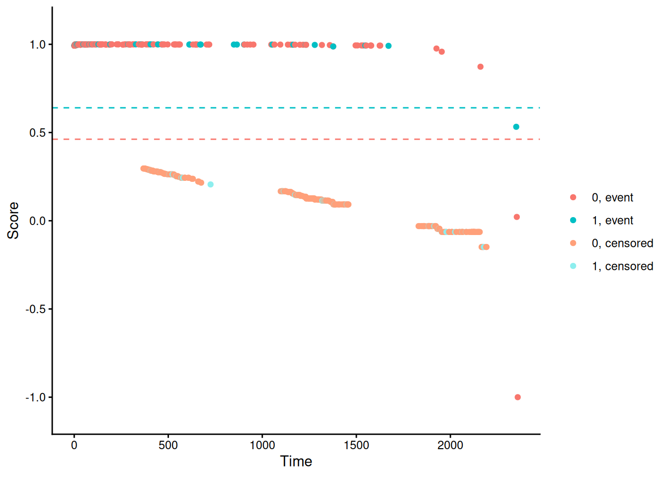
Leton and Zuluaga (2001) illustrated that every weighted log-rank test can be written as either an observed-minus-expected test or as a permutation test. The weights can be reformulated as scores for a permutation test. The scores are obtained from the nphRCT::find_scores function. Plotting these scores against the rank of the event times provides an intuitive understanding of how the weighting operates in the modestly weighted log‑rank test, since the event scores decrease with time, as illustrated by Magirr(2021). Censoring score naturally reduces with time, since it is a negative cumulative sum of increasing weights.

df_scores_mw<-nphRCT::find_scores(formula=Surv(LENFOL,FSTAT)~AFB,
  data=WHAS,
  method="mw",
  s_star = 0.5)
plot(df_scores_mw)

Warning: `aes_string()` was deprecated in ggplot2 3.0.0.
ℹ Please use tidy evaluation idioms with `aes()`.
ℹ See also `vignette("ggplot2-in-packages")` for more information.
ℹ The deprecated feature was likely used in the nphRCT package.
  Please report the issue to the authors.

ii). Stratified Modestly Weighted Log-Rank Test (Stratified MWLRT)

A modestly weighted log-Rank test statistic can be computed separately for the two strata. Here, the stratifying variable is GENDER. The combined test statistic is obtained by combining stratum-specific standardised Z-statistics on the Z-scale using a variance-weighted combination as discussed in Magirr and Jiménez (2022).

smodestly <- nphRCT::wlrt(
  formula = Surv(LENFOL, FSTAT)~AFB + strata(GENDER),data = WHAS,method = "mw",
  s_star = 0.5)
z_strata <- smodestly$by_strata$z
z_combined <- smodestly$combined$z
pchi_sq <- z_strata^2
cchi_sq <- z_combined^2
pp_value <- pchisq(pchi_sq, df = 1, lower.tail = FALSE)
cp_value <- pchisq(cchi_sq, df = 1, lower.tail = FALSE)
cat(sprintf("\nStrata Chi-square: %.6f   p-value: %.6f\n", pchi_sq, pp_value))


Strata Chi-square: 7.518538   p-value: 0.006107
 
Strata Chi-square: 3.741750   p-value: 0.053069

cat(sprintf("\nCombined Chi-square: %.6f   p-value: %.6f\n", cchi_sq, cp_value))


Combined Chi-square: 10.835864   p-value: 0.000996

References

wlrt() documentation: https://search.r-project.org/CRAN/refmans/nphRCT/html/wlrt.html
survdiff() documentation: https://www.rdocumentation.org/packages/survival/versions/3.8-3/topics/survdiff
survminer() documentation: https://cran.r-project.org/web/packages/survminer/survminer.pdf
logrank.maxtest() documentation: https://search.r-project.org/CRAN/refmans/nph/html/logrank.maxtest.html
Robust modestly weighted log-rank testsdocumentation:https://arxiv.org/html/2412.14942v1
nphRCT package documentation: https://cran.r-project.org/web/packages/nphRCT/nphRCT.pdf
Applied survival analysis using R (Vol. 473, pp. 1-10) documentation: https://xsliulab.github.io/Workshop/2021/week3/survival-analysis-book.pdf
Stratified modestly weighted log-rank test documentation: https://cran.r-project.org/web/packages/nphRCT/vignettes/weighted_log_rank_tests.html
Stratified Max-Combo documentation: https://cran.r-project.org/web/packages/strata.MaxCombo/strata.MaxCombo.pdf
Max-combo documentation: https://search.r-project.org/CRAN/refmans/nph/html/logrank.maxtest.html
Modestly weighted log-rank test documentation: https://pubmed.ncbi.nlm.nih.gov/31131462/
Modestly weighted log-rank test documentation: https://arxiv.org/pdf/1807.11097
Modestly weighted log-rank test documentation: https://arxiv.org/pdf/2007.04767v1
Magirr and Jiménez (2022): https://arxiv.org/abs/2201.10445
Magirr, D. (2021) https://onlinelibrary.wiley.com/doi/full/10.1002/pst.2091?msockid=1c39595bd65d63dd3de44ff2d7476288
Leton and Zuluaga (2001) https://www.researchgate.net/publication/243044681_Equivalence_between_score_and_weighted_tests_for_survival_curves

References for other mentioned tests:

Milestone survival. https://cran.r-project.org/web/packages/SingleArmMRCT/vignettes/survival-endpoints.html
Restricted Mean Survival Time (RMST) https://cran.r-project.org/web/packages/simtrial/vignettes/rmst.html

Session Info

─ Session info ───────────────────────────────────────────────────────────────
 setting  value
 version  R version 4.5.2 (2025-10-31)
 os       Ubuntu 24.04.4 LTS
 system   x86_64, linux-gnu
 ui       X11
 language (EN)
 collate  C.UTF-8
 ctype    C.UTF-8
 tz       UTC
 date     2026-05-27
 pandoc   3.8.3 @ /opt/quarto/bin/tools/ (via rmarkdown)

─ Packages ───────────────────────────────────────────────────────────────────
 ! package  * version date (UTC) lib source
 P nphRCT   * 0.1.1   2024-06-27 [?] RSPM (R 4.5.0)
   survival * 3.8-3   2024-12-17 [2] CRAN (R 4.5.2)

 [1] /home/runner/work/CAMIS/CAMIS/renv/library/linux-ubuntu-noble/R-4.5/x86_64-pc-linux-gnu
 [2] /opt/R/4.5.2/lib/R/library

 P ── Loaded and on-disk path mismatch.

──────────────────────────────────────────────────────────────────────────────

Introduction

wlrt()

survdiff()

Data.

Tests:

1. Weighted Log-Rank test.

a). Peto-Peto

i) survminer::surv_pvalue()

ii) coin::logrank_test()

iii) survival::survdiff()

b). Modified Peto-Peto.

i). survminer::surv_pvalue()

ii). coin::logrank_test()

c). Tarone-Ware.

i). survminer::surv_pvalue()

ii) coin::logrank_test()

d). Gehan-Breslow.

i). survminer::surv_pvalue()

ii) coin::logrank_test()

e). Fleming-Harrington

i). nphRCT::wlrt()

ii). coin::logrank_test()

2. Max-Combo test.

i). Max-Combo(No strata)

ii). Stratified Max-Combo

3. Modestly Weighted Log-Rank test.

i). Modestly Weighted Log-rank test(No strata)

ii). Stratified Modestly Weighted Log-Rank Test (Stratified MWLRT)

References

References for other mentioned tests:

i) `survminer::surv_pvalue()`

ii) `coin::logrank_test()`

iii) `survival::survdiff()`

i). `survminer::surv_pvalue()`

ii). `coin::logrank_test()`

i). `survminer::surv_pvalue()`

ii) `coin::logrank_test()`

i). `survminer::surv_pvalue()`

ii) `coin::logrank_test()`

i). `nphRCT::wlrt()`

ii). `coin::logrank_test()`