The most commonly used models for count data in clinical trials include:
Poisson regression: assumes the response variable \(Y\) has a Poisson distribution, which is linked using the logarithm with explanatory variables \(\bf{x}\).
Quasi-Poisson regression: Poisson model that allows overdispersion, i.e. dispersion parameter is not fixed at one.
Negative-Binomial regression: popular generalization which loosens the assumption that the variance is equal to the mean made by the Poisson model.
Other models include hurdle or zero-inflated models, if data have more zero observations than expected.
Example: Familial Andenomatous Polyposis Data
Data source: F. M. Giardiello, S. R. Hamilton, A. J. Krush, S. Piantadosi, L. M. Hylind, P. Celano, S. V. Booker, C. R. Robinson and G. J. A. Offerhaus (1993), Treatment of colonic and rectal adenomas with sulindac in familial adenomatous polyposis. New England Journal of Medicine, 328(18), 1313–1316.
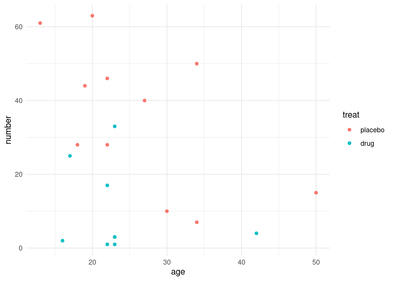
Data from a placebo-controlled trial of a non-steroidal anti-inflammatory drug in the treatment of familial andenomatous polyposis (FAP). (see ?polyps for details).
We analyze the number of colonic polyps at 12 months in dependency of treatment and age of the patient.
polyps |>ggplot(aes(y = number, x = age, color = treat)) +geom_point() +theme_minimal()
Poisson Distribution Models
We fit a generalized linear model for number using the Poisson distribution with default log link.
# Poissonm1 <- stats::glm(number ~ treat + age, data = polyps, family = poisson)summary(m1)
Call:
stats::glm(formula = number ~ treat + age, family = poisson,
    data = polyps)

Coefficients:
             Estimate Std. Error z value Pr(>|z|)
(Intercept)  4.529024   0.146872   30.84  < 2e-16 ***
treatdrug   -1.359083   0.117643  -11.55  < 2e-16 ***
age         -0.038830   0.005955   -6.52 7.02e-11 ***
---
Signif. codes:  0 '***' 0.001 '**' 0.01 '*' 0.05 '.' 0.1 ' ' 1

(Dispersion parameter for poisson family taken to be 1)

    Null deviance: 378.66  on 19  degrees of freedom
Residual deviance: 179.54  on 17  degrees of freedom
AIC: 273.88

Number of Fisher Scoring iterations: 5
The parameter estimates are on log-scale. For better interpretation, we can exponentiate these estimates, to obtain estimates and provide \(95\)% confidence intervals:
# OR and CIexp(coef(m1))
(Intercept)   treatdrug         age
 92.6681047   0.2568961   0.9619140
Predictions for number of colonic polyps given a new 25-year-old patient on either treatment using predict():
# new 25 year old patientnew_pt <-data.frame(treat =c("drug", "placebo"), age =25)predict(m1, new_pt, type ="response")
        1         2
 9.017654 35.102332
Modelling Overdispersion
Quasi Poisson Modelling
Poisson model assumes that mean and variance are equal, which can be a very restrictive assumption. One option to relax the assumption is adding a overdispersion constant to the relationship, i.e. \(\text{Var}(\text{response}) = \phi\cdot \mu\), which results in a quasipoisson model:
# Quasi poissonm2 <- stats::glm(number ~ treat + age, data = polyps, family = quasipoisson)summary(m2)
Call:
stats::glm(formula = number ~ treat + age, family = quasipoisson,
    data = polyps)

Coefficients:
            Estimate Std. Error t value Pr(>|t|)
(Intercept)  4.52902    0.48106   9.415 3.72e-08 ***
treatdrug   -1.35908    0.38533  -3.527  0.00259 **
age         -0.03883    0.01951  -1.991  0.06284 .
---
Signif. codes:  0 '***' 0.001 '**' 0.01 '*' 0.05 '.' 0.1 ' ' 1

(Dispersion parameter for quasipoisson family taken to be 10.72805)

    Null deviance: 378.66  on 19  degrees of freedom
Residual deviance: 179.54  on 17  degrees of freedom
AIC: NA

Number of Fisher Scoring iterations: 5
Negative Binomial Modelling
Alternatively, we can explicitly model the count data with overdispersion using the negative Binomial model. In this case, the overdispersion is a function of both \(\mu\) and \(\mu^2\):
Call:
MASS::glm.nb(formula = number ~ treat + age, data = polyps, init.theta = 1.719491,
    link = log)

Coefficients:
            Estimate Std. Error z value Pr(>|z|)
(Intercept)  4.52603    0.59466   7.611 2.72e-14 ***
treatdrug   -1.36812    0.36903  -3.707 0.000209 ***
age         -0.03856    0.02095  -1.840 0.065751 .
---
Signif. codes:  0 '***' 0.001 '**' 0.01 '*' 0.05 '.' 0.1 ' ' 1

(Dispersion parameter for Negative Binomial(1.7195) family taken to be 1)

    Null deviance: 36.734  on 19  degrees of freedom
Residual deviance: 22.002  on 17  degrees of freedom
AIC: 164.88

Number of Fisher Scoring iterations: 1

              Theta:  1.719
          Std. Err.:  0.607

 2 x log-likelihood:  -156.880
Both model result very similar parameter estimates, but vary in estimates for their respective standard deviation.
Note: the MASS::select() function can cause conflict with the dplyr::select() function. To make your code robust to duplicate functions appearing in different packages, it’s good practice to always include the package name in your code prior to the function. For example, use dplyr::select() instead of just select(), and then if you are using MASS() for negative binomial regression then you wont have a conflict with using select() in other parts of your code!
Negative Binomial Modelling with an offset variable
On clinical trials, subjects are not usually all followed for the full duration of the trial (e.g. for a full 12 months). Instead, it is common to have subjects withdrawing from study or treatment and being impacted by intercurrent events (ICEs) such as rescue medications. This means when we are counting numbers of events, their count may be impacted by the follow up time that we studied them for.
Negative binomial modelling is often adjusted for the follow up time, by including an ‘offset’ variable as shown below.
# Suppose we have a variable with the Follow up period for each subject# We've just created a pretend one below!set.seed(12345)polyps2 <- polyps %>% dplyr::mutate(followup =runif(nrow(.),min=1,max=100)) # Negative Binomial with offset of the follow up time per subjectm3 <- MASS::glm.nb(number ~ treat + age +offset(log(followup)), data = polyps2)summary(m3)
Call:
MASS::glm.nb(formula = number ~ treat + age + offset(log(followup)),
    data = polyps2, init.theta = 0.5594476787, link = log)

Coefficients:
            Estimate Std. Error z value Pr(>|z|)
(Intercept)  2.00562    0.99456   2.017   0.0437 *
treatdrug   -2.86236    0.62679  -4.567 4.96e-06 ***
age         -0.02711    0.03458  -0.784   0.4331
---
Signif. codes:  0 '***' 0.001 '**' 0.01 '*' 0.05 '.' 0.1 ' ' 1

(Dispersion parameter for Negative Binomial(0.5594) family taken to be 1)

    Null deviance: 39.165  on 19  degrees of freedom
Residual deviance: 24.462  on 17  degrees of freedom
AIC: 190.33

Number of Fisher Scoring iterations: 1

              Theta:  0.559
          Std. Err.:  0.155

 2 x log-likelihood:  -182.330