Multiple Imputaton: Linear Regression

Overview

Multiple imputation with regression is one step further from mean imputation (i.e. by a single value: the average of observed). In the case for continuous, normally distributed variable, linear regression can use information from other variables hence could be closer to the true missing values.

Imputation with mice

mice is a powerful R package developed by Stef van Buuren, Karin Groothuis-Oudshoorn and other contributors. Regression methods (continuous, normal outcome) are implemented in mice with methods starting with norm.

Example

Here I use the small dataset nhanes included in mice package. It has 25 rows, and three out of four variables have missings.

The original NHANES data is a large national level survey, some are publicly available via R package nhanes.

library(mice)

Attaching package: 'mice'
The following object is masked from 'package:stats':

    filter
The following objects are masked from 'package:base':

    cbind, rbind
# load example dataset from mice
head(nhanes)
  age  bmi hyp chl
1   1   NA  NA  NA
2   2 22.7   1 187
3   1   NA   1 187
4   3   NA  NA  NA
5   1 20.4   1 113
6   3   NA  NA 184
summary(nhanes)
      age            bmi             hyp             chl       
 Min.   :1.00   Min.   :20.40   Min.   :1.000   Min.   :113.0  
 1st Qu.:1.00   1st Qu.:22.65   1st Qu.:1.000   1st Qu.:185.0  
 Median :2.00   Median :26.75   Median :1.000   Median :187.0  
 Mean   :1.76   Mean   :26.56   Mean   :1.235   Mean   :191.4  
 3rd Qu.:2.00   3rd Qu.:28.93   3rd Qu.:1.000   3rd Qu.:212.0  
 Max.   :3.00   Max.   :35.30   Max.   :2.000   Max.   :284.0  
                NA's   :9       NA's   :8       NA's   :10     

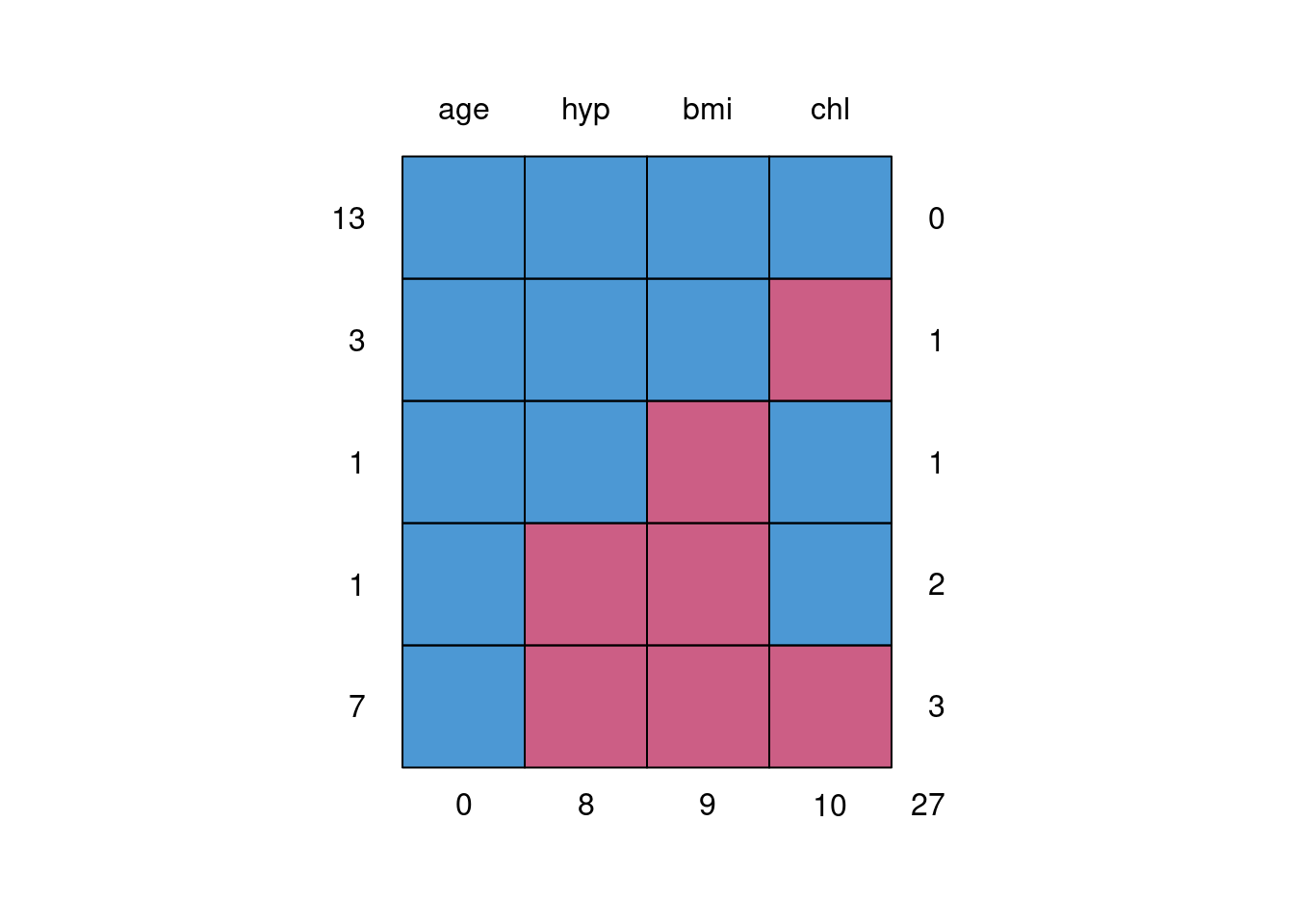
Examine missing pattern with md.pattern(data).

# 27 missing in total
# by col: 8 for hyp, 9 for bmi, 10 for chl
# by row: n missing numbers

md.pattern(nhanes)

   age hyp bmi chl   
13   1   1   1   1  0
3    1   1   1   0  1
1    1   1   0   1  1
1    1   0   0   1  2
7    1   0   0   0  3
     0   8   9  10 27

Regression without parameter uncertainty

We can generate two imputed datasets by setting m=2.

There is a certain level of randomness, so would be a good idea to set seed.

set.seed(1)
impr0 <- mice(nhanes, method = 'norm.nob', m=2, maxit = 1)

 iter imp variable
  1   1  bmi  hyp  chl
  1   2  bmi  hyp  chl
impr0
Class: mids
Number of multiple imputations:  2 
Imputation methods:
       age        bmi        hyp        chl 
        "" "norm.nob" "norm.nob" "norm.nob" 
PredictorMatrix:
    age bmi hyp chl
age   0   1   1   1
bmi   1   0   1   1
hyp   1   1   0   1
chl   1   1   1   0
nhanes_impr0 <- complete(impr0) # by default, returns the first imputation
nhanes_impr0
   age      bmi       hyp      chl
1    1 35.53430 1.2503841 256.6153
2    2 22.70000 1.0000000 187.0000
3    1 27.31412 1.0000000 187.0000
4    3 25.31243 2.3880837 267.1435
5    1 20.40000 1.0000000 113.0000
6    3 17.94547 1.5855064 184.0000
7    1 22.50000 1.0000000 118.0000
8    1 30.10000 1.0000000 187.0000
9    2 22.00000 1.0000000 238.0000
10   2 26.99782 1.0810473 206.9927
11   1 32.71511 0.7819353 213.7222
12   2 27.65399 0.7904680 209.6716
13   3 21.70000 1.0000000 206.0000
14   2 28.70000 2.0000000 204.0000
15   1 29.60000 1.0000000 252.1596
16   1 27.47980 0.6071353 145.9557
17   3 27.20000 2.0000000 284.0000
18   2 26.30000 2.0000000 199.0000
19   1 35.30000 1.0000000 218.0000
20   3 25.50000 2.0000000 245.7884
21   1 35.12809 0.5807116 232.4652
22   1 33.20000 1.0000000 229.0000
23   1 27.50000 1.0000000 131.0000
24   3 24.90000 1.0000000 268.3929
25   2 27.40000 1.0000000 186.0000

When we have two imputed datasets, we can check the values for each of the variables. For example, extract bmi variable from the imputed data imp,

# two imputed datasets (m=2)
impr0$imp$bmi
          1        2
1  35.53430 32.26078
3  27.31412 22.55473
4  25.31243 14.90410
6  17.94547 22.59196
10 26.99782 25.08534
11 32.71511 27.71485
12 27.65399 25.76286
16 27.47980 30.34985
21 35.12809 29.89142

We can also specify which imputed dataset to use as our complete data. Set index to 0 (action = 0) returns the original dataset with missing values.

Here we check which of the imputed data is being used as the completed dataset. First take a note of the row IDs (based on bmi, for example). Then we generate completed dataset.

  • if no action argument is set, then it returns the first imputation by default
  • action=0 corresponds to the original data with missing values
# check which imputed data is used for the final result, take note of row id
id_missing <- which(is.na(nhanes$bmi))
id_missing
[1]  1  3  4  6 10 11 12 16 21
nhanes_impr0_action0 <- complete(impr0, action = 0) 
nhanes_impr0_action0[id_missing, ] # original data with missing bmi
   age bmi hyp chl
1    1  NA  NA  NA
3    1  NA   1 187
4    3  NA  NA  NA
6    3  NA  NA 184
10   2  NA  NA  NA
11   1  NA  NA  NA
12   2  NA  NA  NA
16   1  NA  NA  NA
21   1  NA  NA  NA
nhanes_impr0_action1 <- complete(impr0, action = 1) 
nhanes_impr0_action1[id_missing, ] # using first imputation
   age      bmi       hyp      chl
1    1 35.53430 1.2503841 256.6153
3    1 27.31412 1.0000000 187.0000
4    3 25.31243 2.3880837 267.1435
6    3 17.94547 1.5855064 184.0000
10   2 26.99782 1.0810473 206.9927
11   1 32.71511 0.7819353 213.7222
12   2 27.65399 0.7904680 209.6716
16   1 27.47980 0.6071353 145.9557
21   1 35.12809 0.5807116 232.4652
nhanes_impr0_action2 <- complete(impr0, action = 2) 
nhanes_impr0_action2[id_missing, ] # using second imputation
   age      bmi       hyp      chl
1    1 32.26078 0.4616324 228.0022
3    1 22.55473 1.0000000 187.0000
4    3 14.90410 1.4558818 212.7958
6    3 22.59196 1.7664882 184.0000
10   2 25.08534 1.2940549 201.5872
11   1 27.71485 0.9410698 169.2427
12   2 25.76286 1.3570093 168.5961
16   1 30.34985 0.6878971 163.7262
21   1 29.89142 1.0452062 212.9144

Other imputation by linear regression

Other various of imputaton via linear regression can be implemented simply by changing the method argument.

impr <- mice(nhanes, method = 'norm.predict', m=1, maxit=1)

 iter imp variable
  1   1  bmi  hyp  chl
impr$imp$bmi
          1
1  28.33396
3  28.33396
4  22.75613
6  21.17519
10 27.19573
11 29.12443
12 26.26576
16 30.28688
21 28.33396

Bayesian linear regression

impb <- mice(nhanes, method = 'norm', m=1, maxit=1)

 iter imp variable
  1   1  bmi  hyp  chl
impb$imp$bmi
          1
1  33.82959
3  28.98754
4  20.88810
6  19.11391
10 27.32990
11 29.44117
12 22.68062
16 32.13267
21 22.03164
# nhanes_impb <- complete(impb)

Bootstrap

impbt <- mice(nhanes, method = 'norm.boot', m=1, maxit=1)

 iter imp variable
  1   1  bmi  hyp  chl
impbt$imp$bmi
          1
1  24.19248
3  28.77464
4  22.42321
6  23.47542
10 21.95529
11 23.12703
12 25.84230
16 27.68216
21 26.43770

Reference

Stef van Buuren, Karin Groothuis-Oudshoorn (2011). mice: Multivariate Imputation by Chained Equations in R. Journal of Statistical Software, 45(3), 1-67. DOI 10.18637/jss.v045.i03