# General
library(dplyr)
library(tidyr)
library(gt)
library(labelled)

# Methodlolgy specific
library(mmrm)
library(emmeans)
library(rbmi)
library(mice) # only used md.pattern()Reference-Based Multiple Imputation (joint modelling): Continuous Data
Libraries
Reference-based multiple imputation (rbmi)
Methodology introduction
Reference-based multiple imputation methods have become popular for handling missing data, as well as for conducting sensitivity analyses, in randomized clinical trials. In the context of a repeatedly measured continuous endpoint assuming a multivariate normal model, Carpenter et al. (2013) proposed a framework to extend the usual MAR-based MI approach by postulating assumptions about the joint distribution of pre- and post-deviation data. Under this framework, one makes qualitative assumptions about how individuals’ missing outcomes relate to those observed in relevant groups in the trial, based on plausible clinical scenarios. Statistical analysis then proceeds using the method of multiple imputation (Rubin 1976, Rubin 1987).
In general, multiple imputation of a repeatedly measured continuous outcome can be done via 2 computational routes (Roger 2022):
Stepwise: split problem into separate imputations of data at each visit
requires monotone missingness, such as missingness due to withdrawal
conditions on the imputed values at previous visit
Bayesian linear regression problem is much simpler with monotone missing, as one can sample directly using conjugate priors
One-step approach (joint modelling): Fit a Bayesian full multivariate normal repeated measures model using MCMC and then draw a sample.
Here, we illustrate reference-based multiple imputation of a continuous outcome measured repeatedly via the so-called one-step approach.
rbmi package
The rbmi package Gower-Page et al. (2022) will be used for the one-step approach of the reference-based multiple imputation using R. The package implements standard and reference based multiple imputation methods for continuous longitudinal endpoints . In particular, this package supports deterministic conditional mean imputation and jackknifing as described in Wolbers et al. (2022), convential MI based on Bayesian posterior draws as described in Carpenter et al. (2013), and bootstrapped maximum likelihood imputation as described in von Hippel and Bartlett (2021).
The following standard and reference-based multiple imputation approaches will be illustrated here:
* MAR (Missing At Random)

* CIR (Copy Increment from Reference)

* J2R (Jump to Reference)

* CR (Copy Reference)
Data used
A publicly available example dataset from an antidepressant clinical trial of an active drug versus placebo is used. Overall, data of 172 patients is available with 88 patients receiving placebo and 84 receiving active drug. This data is also used in the rbmi package quickstart vignette.
The relevant endpoint is the Hamilton 17-item depression rating scale (HAMD17) which was assessed at baseline and at weeks 1, 2, 4, and 6 (visits 4-7). Study drug discontinuation occurred in 24% (20/84) of subjects from the active drug and 26% (23/88) of subjects from placebo. All data after study drug discontinuation are missing.
data("antidepressant_data")
dat <- antidepressant_data |>
  dplyr::select(
    PATIENT,
    GENDER,
    THERAPY,
    RELDAYS,
    VISIT,
    BASVAL,
    HAMDTL17,
    CHANGE
  ) |>
  dplyr::mutate(THERAPY = factor(THERAPY, levels = c("PLACEBO", "DRUG"))) |>
  labelled::remove_labels()

gt(head(dat, n = 10))| PATIENT | GENDER | THERAPY | RELDAYS | VISIT | BASVAL | HAMDTL17 | CHANGE |
|---|---|---|---|---|---|---|---|
| 1503 | F | DRUG | 7 | 4 | 32 | 21 | -11 |
| 1503 | F | DRUG | 14 | 5 | 32 | 20 | -12 |
| 1503 | F | DRUG | 28 | 6 | 32 | 19 | -13 |
| 1503 | F | DRUG | 42 | 7 | 32 | 17 | -15 |
| 1507 | F | PLACEBO | 7 | 4 | 14 | 11 | -3 |
| 1507 | F | PLACEBO | 15 | 5 | 14 | 14 | 0 |
| 1507 | F | PLACEBO | 29 | 6 | 14 | 9 | -5 |
| 1507 | F | PLACEBO | 42 | 7 | 14 | 5 | -9 |
| 1509 | F | DRUG | 7 | 4 | 21 | 20 | -1 |
| 1509 | F | DRUG | 14 | 5 | 21 | 18 | -3 |
The number of patients per visit and arm are:
dat |>
  group_by(VISIT, THERAPY) |>
  dplyr::summarise(N = n())
`summarise()` has regrouped the output.
ℹ Summaries were computed grouped by VISIT and THERAPY.
ℹ Output is grouped by VISIT.
ℹ Use `summarise(.groups = "drop_last")` to silence this message.
ℹ Use `summarise(.by = c(VISIT, THERAPY))` for per-operation grouping
(`?dplyr::dplyr_by`) instead.# A tibble: 8 × 3
# Groups: VISIT [4]
VISIT THERAPY N
<fct> <fct> <int>
1 4 PLACEBO 88
2 4 DRUG 84
3 5 PLACEBO 81
4 5 DRUG 77
5 6 PLACEBO 76
6 6 DRUG 73
7 7 PLACEBO 65
8 7 DRUG 64The mean change from baseline of the endpoint (Hamilton 17-item depression rating scale, HAMD17) per visit per treatment group using only the complete cases are:
dat |>
  group_by(VISIT, THERAPY) |>
  dplyr::summarise(N = n(), MEAN = mean(CHANGE))
`summarise()` has regrouped the output.
ℹ Summaries were computed grouped by VISIT and THERAPY.
ℹ Output is grouped by VISIT.
ℹ Use `summarise(.groups = "drop_last")` to silence this message.
ℹ Use `summarise(.by = c(VISIT, THERAPY))` for per-operation grouping
(`?dplyr::dplyr_by`) instead.# A tibble: 8 × 4
# Groups: VISIT [4]
VISIT THERAPY N MEAN
<fct> <fct> <int> <dbl>
1 4 PLACEBO 88 -1.51
2 4 DRUG 84 -1.82
3 5 PLACEBO 81 -2.70
4 5 DRUG 77 -4.71
5 6 PLACEBO 76 -4.07
6 6 DRUG 73 -6.79
7 7 PLACEBO 65 -5.14
8 7 DRUG 64 -8.34The missingness pattern is show below (1=observed data point (blue), 0=missing data point (red)). The incomplete data is primarily monotone in nature. 128 patients have complete data for all visits (all 1’s at each visit). 20, 10 and 13 patients have 1, 2 or 3 monotone missing data, respectively. Further, there is a single additional intermittent missing observation (patient 3618).
dat_wide = dat |>
  dplyr::select(PATIENT, VISIT, CHANGE) |>
  pivot_wider(
    id_cols = PATIENT,
    names_from = VISIT,
    names_prefix = "VISIT_",
    values_from = CHANGE
  )

dat_wide |>
  dplyr::select(starts_with("VISIT_")) |>
  mice::md.pattern(plot = TRUE, rotate.names = TRUE)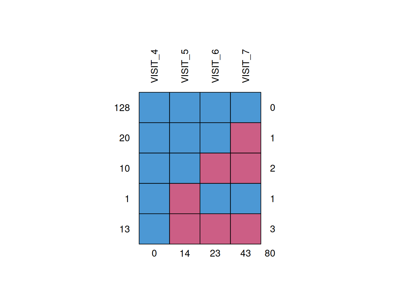
    VISIT_4 VISIT_5 VISIT_6 VISIT_7
128       1       1       1       1  0
20        1       1       1       0  1
10        1       1       0       0  2
1         1       0       1       1  1
13        1       0       0       0  3
          0      14      23      43 80
Complete case analysis
A complete case analysis is performed using mixed model for repeated measures (MMRM) with covariates: treatment [THERAPY], gender [GENDER], visit [VISIT] as factors; baseline score [BASVAL] as continuous; and visit-by-treatment [THERAPY * VISIT] interaction, and visit-by-baseline [BASVAL * VISIT] interaction. An unstructured covariance matrix is used.
mmrm_fit = mmrm::mmrm(
  CHANGE ~
    1 +
      THERAPY +
      GENDER +
      VISIT +
      BASVAL +
      THERAPY * VISIT +
      BASVAL * VISIT +
      us(VISIT | PATIENT),
  data = dat,
  reml = TRUE
)
summary(mmrm_fit)
mmrm fit
Formula:
CHANGE ~ 1 + THERAPY + GENDER + VISIT + BASVAL + THERAPY * VISIT +
BASVAL * VISIT + us(VISIT | PATIENT)
Data: dat (used 608 observations from 172 subjects with maximum 4
timepoints)
Covariance: unstructured (10 variance parameters)
Method: Satterthwaite
Vcov Method: Asymptotic
Inference: REML
Model selection criteria:
AIC BIC logLik deviance
3512.9 3544.4 -1746.5 3492.9
Coefficients:
Estimate Std. Error df t value Pr(>|t|)
(Intercept) 3.16355 1.20260 168.64000 2.631 0.00931 **
THERAPYDRUG 0.06603 0.68662 168.11000 0.096 0.92350
GENDERM 0.31961 0.68216 168.46000 0.469 0.64001
VISIT5 -0.50646 1.22706 157.16000 -0.413 0.68036
VISIT6 -0.39390 1.41983 149.35000 -0.277 0.78184
VISIT7 -2.29237 1.62198 142.91000 -1.413 0.15974
BASVAL -0.27866 0.06222 168.05000 -4.479 1.38e-05 ***
THERAPYDRUG:VISIT5 -1.49495 0.73342 156.86000 -2.038 0.04320 *
THERAPYDRUG:VISIT6 -2.31710 0.85860 151.23000 -2.699 0.00775 **
THERAPYDRUG:VISIT7 -2.89468 0.96582 139.86000 -2.997 0.00323 **
VISIT5:BASVAL -0.03429 0.06567 157.48000 -0.522 0.60231
VISIT6:BASVAL -0.11482 0.07646 150.73000 -1.502 0.13527
VISIT7:BASVAL -0.04656 0.08679 142.04000 -0.537 0.59244
---
Signif. codes: 0 '***' 0.001 '**' 0.01 '*' 0.05 '.' 0.1 ' ' 1
Covariance estimate:
4 5 6 7
4 19.7877 16.6237 15.4265 16.4578
5 16.6237 34.3231 25.4682 26.2897
6 15.4265 25.4682 38.4094 33.9331
7 16.4578 26.2897 33.9331 45.3625Using the emmeans package/function least square means and contrast can be obtained.
em = emmeans::emmeans(
  mmrm_fit,
  specs = trt.vs.ctrl ~ THERAPY * VISIT,
  at = list(VISIT = "7"),
  level = 0.95,
  adjust = "none",
  mode = "df.error"
)

em_contrast = broom::tidy(em$contrasts, conf.int = TRUE, conf.level = 0.95)
em_contrast |>
  gt() |>
fmt_number(decimals = 3)| term | contrast | null.value | estimate | std.error | df | conf.low | conf.high | statistic | p.value |
|---|---|---|---|---|---|---|---|---|---|
| THERAPY*VISIT | DRUG VISIT7 - PLACEBO VISIT7 | 0.000 | −2.829 | 1.117 | 150.711 | −5.035 | −0.622 | −2.533 | 0.012 |
The treatment difference at visit 7 is of interest, and is estimated to be -2.829 (se=1.117) with 95% CI of [-5.035 to -0.622] (p=0.0123).
rbmi: MAR approach
The code presented here is based on the rbmi package quickstart vignette.
Create needed datasets and specify imputation strategy
rbmi expects its input dataset to be complete; that is, there must be one row per subject for each visit (note: in clinical trials ADAMs typically do not have this required complete data structure). Missing outcome values should be coded as NA, while missing covariate values are not allowed. If the dataset is incomplete, then the expand_locf() function can be used to add any missing rows, using LOCF imputation to carry forward the observed baseline covariate values to visits with missing outcomes.
dat_expand <- rbmi::expand_locf(
  dat,
  PATIENT = levels(dat$PATIENT), # expand by PATIENT and VISIT
  VISIT = levels(dat$VISIT),
  vars = c("BASVAL", "THERAPY", "GENDER"), # complete covariates using LOCF
  group = c("PATIENT"),
  order = c("PATIENT", "VISIT") # sort
)
For example, the data of patient 1513 in the original data and expanded data are:
dat |>
  dplyr::filter(PATIENT == "1513") |>
gt()| PATIENT | GENDER | THERAPY | RELDAYS | VISIT | BASVAL | HAMDTL17 | CHANGE |
|---|---|---|---|---|---|---|---|
| 1513 | M | DRUG | 7 | 4 | 19 | 24 | 5 |
dat_expand |>
  dplyr::filter(PATIENT == "1513") |>
gt()| PATIENT | GENDER | THERAPY | RELDAYS | VISIT | BASVAL | HAMDTL17 | CHANGE |
|---|---|---|---|---|---|---|---|
| 1513 | M | DRUG | 7 | 4 | 19 | 24 | 5 |
| 1513 | M | DRUG | NA | 5 | 19 | NA | NA |
| 1513 | M | DRUG | NA | 6 | 19 | NA | NA |
| 1513 | M | DRUG | NA | 7 | 19 | NA | NA |
Next, a dataset must be created specifying which data points should be imputed with the specified imputation strategy. The dataset dat_ice is created which specifies the first visit affected by an intercurrent event (ICE) and the imputation strategy for handling missing outcome data after the ICE. At most one ICE which is to be imputed is allowed per subject. In the example, the subject’s first visit affected by the ICE “study drug discontinuation” corresponds to the first terminal missing observation
dat_ice <- dat_expand |>
  arrange(PATIENT, VISIT) |>
  filter(is.na(CHANGE)) |>
  group_by(PATIENT) |>
  slice(1) |>
  ungroup() |>
  select(PATIENT, VISIT) |>
  mutate(strategy = "MAR")

gt(head(dat_ice))| PATIENT | VISIT | strategy |
|---|---|---|
| 1513 | 5 | MAR |
| 1514 | 5 | MAR |
| 1517 | 5 | MAR |
| 1804 | 7 | MAR |
| 2104 | 7 | MAR |
| 2118 | 5 | MAR |
In this dataset, subject 3618 has an intermittent missing values which does not correspond to a study drug discontinuation. We therefore remove this subject from dat_ice. In the later imputation step, it will automatically be imputed under the default MAR assumption.
dat_ice <- dat_ice[-which(dat_ice$PATIENT == 3618), ]Fit imputation model and draw posterior parameters
The vars object using using set_vars() defines the names of key variables in the dataset and the covariates included in the imputation model. If you wish to include interaction terms these need to be added in the covariates input.
The method object specifies the statistical method used to fit the imputation models and to create imputed datasets.
The draws() function fits the imputation model and stores the corresponding parameter estimates and Bayesian posterior parameter draws.
vars <- rbmi::set_vars(
  outcome = "CHANGE",
  visit = "VISIT",
  subjid = "PATIENT",
  group = "THERAPY",
  covariates = c("GENDER", "BASVAL*VISIT", "THERAPY*VISIT")
)

method <- rbmi::method_bayes(
  n_samples = 500,
  control = rbmi::control_bayes(warmup = 500, thin = 10)
)

set.seed(12345)
drawObj <- draws(
  data = dat_expand,
  data_ice = dat_ice,
  vars = vars,
  method = method,
  quiet = TRUE
)

drawObj
Draws Object
------------
Number of Samples: 500
Number of Failed Samples: 0
Model Formula: CHANGE ~ 1 + THERAPY + VISIT + GENDER + BASVAL * VISIT + THERAPY * VISIT
Imputation Type: random
Method:
    name: Bayes
    covariance: us
    same_cov: TRUE
    n_samples: 500
    prior_cov: default
Controls:
    warmup: 500
    thin: 10
    chains: 1
    init: mmrm
    seed: 824960212
Generate imputed datasets
The next step is to use the parameters from the imputation model to generate the imputed datasets. This is done via the impute() function. The function only has two key inputs: the imputation model output from draws() and the references groups relevant to reference-based imputation methods. Since we are using the MAR approach here, we can set it to NULL.
imputeObj <- rbmi::impute(draws = drawObj, references = NULL)In case we would like to access the imputed datasets, we can use the extract_imputed_dfs() function. For example, the imputed values in the 10th imputed dataset for patient 1513 are:
imputed_dfs = rbmi::extract_imputed_dfs(imputeObj)
MI_10 = imputed_dfs[[10]]
MI_10$PATIENT_ID = dat_expand$PATIENT

MI_10 |>
  dplyr::filter(PATIENT_ID == "1513") |>
gt()| PATIENT | GENDER | THERAPY | RELDAYS | VISIT | BASVAL | HAMDTL17 | CHANGE | PATIENT_ID |
|---|---|---|---|---|---|---|---|---|
| new_pt_5 | M | DRUG | 7 | 4 | 19 | 24 | 5.000000 | 1513 |
| new_pt_5 | M | DRUG | NA | 5 | 19 | NA | 4.152321 | 1513 |
| new_pt_5 | M | DRUG | NA | 6 | 19 | NA | -11.187646 | 1513 |
| new_pt_5 | M | DRUG | NA | 7 | 19 | NA | -10.287014 | 1513 |
Analyse imputed datasets
The next step is to run the analysis model on each imputed dataset. This is done by defining an analysis function and then calling the analyse() function to apply this function to each imputed dataset. The ancova() function provided by the rbmi package which fits a separate ANCOVA model for the outcomes from each visit is used.
The ancova() function uses the set_vars() function which determines the names of the key variables within the data and the covariates (in addition to the treatment group) for which the analysis model will be adjusted.
Note: In Appendix 1 below we show how you can easily use a different analysis method (e.g., mmrm).
vars_analyse <- rbmi::set_vars(
  outcome = "CHANGE",
  visit = "VISIT",
  subjid = "PATIENT",
  group = "THERAPY",
  covariates = c("BASVAL", "GENDER")
)

anaObj <- rbmi::analyse(
  imputations = imputeObj,
  fun = ancova,
  vars = vars_analyse
)
Pool results
Finally, the pool() function can be used to summarise the analysis results across multiple imputed datasets to provide an overall statistic with a standard error, confidence intervals and a p-value for the hypothesis test of the null hypothesis that the effect is equal to 0. Since we used method_bayes(), pooling and inference are based on Rubin’s rules.
Here, the treatment difference at visit 7 is of interest. Since we set PLACEBO as the first factor in the variable THERAPY this corresponds to ref, whereas DRUG corresponds to alt.
poolObj <- rbmi::pool(anaObj, conf.level = 0.95, alternative = "two.sided")

poolObj |>
  data.frame() |>
  dplyr::filter(grepl("7", parameter)) |>
gt()| parameter | est | se | lci | uci | pval |
|---|---|---|---|---|---|
| trt_7 | -2.816890 | 1.1167760 | -5.024381 | -0.6093975 | 1.275097e-02 |
| lsm_ref_7 | -4.815083 | 0.7780929 | -6.353197 | -3.2769687 | 6.118720e-09 |
| lsm_alt_7 | -7.631972 | 0.7908552 | -9.195110 | -6.0688350 | 2.580413e-17 |
rbmi: MNAR CR approach
The following changes need to be made in the code above to apply the Copy Reference (CR) approach in rbmi. For dat_ice the strategy need to be changed to CR. In the impute() step the references need to be specified. Here we set the reference for the DRUG group to PLACEBO.
dat_ice <- dat_expand |>
  arrange(PATIENT, VISIT) |>
  filter(is.na(CHANGE)) |>
  group_by(PATIENT) |>
  slice(1) |>
  ungroup() |>
  select(PATIENT, VISIT) |>
  mutate(strategy = "CR")

imputeObj <- rbmi::impute(
  drawObj,
  references = c("PLACEBO" = "PLACEBO", "DRUG" = "PLACEBO")
)
The results for M=500 imputed datasets using the MNAR CR approach are:
poolObj |>
  data.frame() |>
  dplyr::filter(grepl("7", parameter)) |>
gt()| parameter | est | se | lci | uci | pval |
|---|---|---|---|---|---|
| trt_7 | -2.393318 | 1.1092180 | -4.585247 | -0.2013897 | 3.256562e-02 |
| lsm_ref_7 | -4.817661 | 0.7796982 | -6.358748 | -3.2765740 | 6.224847e-09 |
| lsm_alt_7 | -7.210979 | 0.7955835 | -8.783369 | -5.6385891 | 7.801168e-16 |
rbmi: MNAR JR approach
The following changes need to be made in the code above to apply the Jump to Reference (JR) approach in rbmi. For dat_ice the strategy need to be changed to JR. In the impute() step the references need to be specified. Here we set the reference for the DRUG group to PLACEBO.
dat_ice <- dat_expand |>
  arrange(PATIENT, VISIT) |>
  filter(is.na(CHANGE)) |>
  group_by(PATIENT) |>
  slice(1) |>
  ungroup() |>
  select(PATIENT, VISIT) |>
  mutate(strategy = "JR")

imputeObj <- rbmi::impute(
  drawObj,
  references = c("PLACEBO" = "PLACEBO", "DRUG" = "PLACEBO")
)
The results for M=500 imputed datasets using the MNAR JR approach are:
poolObj |>
  data.frame() |>
  dplyr::filter(grepl("7", parameter)) |>
gt()| parameter | est | se | lci | uci | pval |
|---|---|---|---|---|---|
| trt_7 | -2.143437 | 1.1269939 | -4.370822 | 0.08394779 | 5.915888e-02 |
| lsm_ref_7 | -4.821702 | 0.7905712 | -6.384460 | -3.25894477 | 9.511139e-09 |
| lsm_alt_7 | -6.965139 | 0.8185475 | -8.583534 | -5.34674432 | 2.496563e-14 |
rbmi: MNAR CIR approach
The following changes need to be made in the code above to apply the Copy Increments in Reference (CIR) approach in rbmi. For dat_ice the strategy need to be changed to CIR. In the impute() step the references need to be specified. Here we set the reference for the DRUG group to PLACEBO.
dat_ice <- dat_expand |>
  arrange(PATIENT, VISIT) |>
  filter(is.na(CHANGE)) |>
  group_by(PATIENT) |>
  slice(1) |>
  ungroup() |>
  select(PATIENT, VISIT) |>
  mutate(strategy = "CIR")

imputeObj <- rbmi::impute(
  drawObj,
  references = c("PLACEBO" = "PLACEBO", "DRUG" = "PLACEBO")
)
The results for M=500 imputed datasets using the MNAR CIR approach are:
poolObj |>
  data.frame() |>
  dplyr::filter(grepl("7", parameter)) |>
gt()| parameter | est | se | lci | uci | pval |
|---|---|---|---|---|---|
| trt_7 | -2.474382 | 1.1080177 | -4.663971 | -0.2847918 | 2.703976e-02 |
| lsm_ref_7 | -4.814550 | 0.7842418 | -6.364835 | -3.2642656 | 7.837117e-09 |
| lsm_alt_7 | -7.288932 | 0.7952036 | -8.860613 | -5.7172516 | 4.368826e-16 |
Summary of results
In the table we present the results of the different imputation strategies (and with varying number, M, of multiple imputation draws). Note that the results can be (slightly) different from the results above due to a possible different seed. The table show the contrast at Visit 7 between DRUG and PLACEBO [DRUG - PLACEBO]:
| Method | Estimate | SE | 95% CI | p-value |
|---|---|---|---|---|
| Complete Case | -2.829 | 1.117 | -5.035 to -0.622 | 0.0123 |
| MI - MAR (M=500) | -2.833 | 1.120 | -5.046 to -0.620 | 0.0125 |
| MI - MAR (M=2000) | -2.837 | 1.118 | -5.047 to -0.627 | 0.0122 |
| MI - MAR (M=5000) | -2.830 | 1.123 | -5.040 to -0.610 | 0.0128 |
| MI - MNAR CR (M=500) | -2.377 | 1.119 | -4.588 to -0.167 | 0.0352 |
| MI - MNAR CR (M=2000) | -2.391 | 1.110 | -4.585 to -0.198 | 0.0328 |
| MI - MNAR CR (M=5000) | -2.394 | 1.112 | -4.592 to -0.197 | 0.0329 |
| MI - MNAR JR (M=500) | -2.169 | 1.134 | -4.411 to 0.072 | 0.0577 |
| MI - MNAR JR (M=2000) | -2.146 | 1.135 | -4.389 to 0.097 | 0.0606 |
| MI - MNAR JR (M=5000) | -2.148 | 1.135 | -4.390 to 0.095 | 0.0603 |
| MI - MNAR CIR (M=500) | -2.495 | 1.113 | -4.695 to -0.295 | 0.0265 |
| MI - MNAR CIR (M=2000) | -2.469 | 1.116 | -4.674 to -0.263 | 0.0285 |
| MI - MNAR CIR (M=5000) | -2.479 | 1.112 | -4.676 to -0.282 | 0.0273 |
Approximate Bayesian
In the draws() function it is possible to specify other methods. For example, the approximate Bayesian MI method_approxbayes() which is based on bootstrapping. draws() returns the draws from the posterior distribution of the parameters using an approximate Bayesian approach, where the sampling from the posterior distribution is simulated by fitting the MMRM model on bootstrap samples of the original dataset.
method <- rbmi::method_approxbayes(
  covariance = "us",
  threshold = 0.01,
  REML = TRUE,
  n_samples = 500
)
In the table we present the results of the approximate Bayesian approach for a CR imputation strategy. The table show the contrast at Visit 7 between DRUG and PLACEBO [DRUG - PLACEBO]:
| Method | Estimate | SE | 95% CI | p-value |
|---|---|---|---|---|
| MI - MNAR CR (M=500) | -2.415 | 1.109 | -4.617 to -0.210 | 0.0320 |
| MI - MNAR CR (M=2000) | -2.403 | 1.112 | -4.600 to -0.205 | 0.0323 |
Discussion
A note on computational time: The total running time (including data loading, setting up data sets, MCMC run, imputing data and analysis MI data) for M=500 was about 26 seconds on a personal laptop. It increased to about 92 seconds for M=2000. Computational time was similar across different imputation strategies.
With a small number of n_samples in method_bayes() a warning could pop-up “The largest R-hat is 1.08, indicating chains have not mixed. Running the chains for more iterations may help”. Increasing the number of n_samples will mostly solve this warning. For example, for this data example, this message is received when setting n_samples equal to a number below 100.
Appendix 1: mmrm as analysis model
In the analyse() function (at the moment of writing) the only available analysis function is ancova. However, the user is able to specify its own analysis function. See the analyse() function for more details.
Another possibility (although, not the most efficient) is to implement a for loop in which the model is fit on each imputed dataset. The obtained results could then be pooled using Rubin’s rule. For example, suppose an MMRM should be fit on each imputed dataset:
mmrm_analyse_mi_function <- function(Impute_Obj) {
  # create all imputed datasets
  imputed_dfs = rbmi::extract_imputed_dfs(Impute_Obj)

  # create empty vectors to store mmrm analysis results
  est_vec = sd_vec = df_vec = NULL

  # for loop to save estimates per imputation
  for (k in 1:length(imputed_dfs)) {
    temp_dat = imputed_dfs[[k]]
    mmrm_fit_temp = mmrm::mmrm(
      CHANGE ~
        1 +
          THERAPY +
          VISIT +
          BASVAL * VISIT +
          THERAPY * VISIT +
          GENDER +
          us(VISIT | PATIENT),
      data = temp_dat,
      reml = TRUE
    )
    em = emmeans::emmeans(
      mmrm_fit_temp,
      specs = trt.vs.ctrl ~ THERAPY * VISIT,
      at = list(VISIT = "7"),
      level = 0.95,
      adjust = "none",
      mode = "df.error"
    )
    est_vec[k] = summary(em$contrasts)$estimate
    sd_vec[k] = summary(em$contrasts)$SE
    df_vec[k] = summary(em$contrasts)$df
  }

  # summarize results using rubin's rule
  rr = rbmi:::rubin_rules(ests = est_vec, ses = sd_vec, v_com = mean(df_vec))
  rr$se_t = sqrt(rr$var_t)
  rr$t.stat = rr$est_point / sqrt(rr$var_t)
  rr$p_value = 2 * pt(q = rr$t.stat, df = rr$df, lower.tail = TRUE)

  return(rr = rr)
}
The following code then performs the analysis and pooling
mmrm_analyse_mi_function(Impute_Obj = imputeObj)In the table we present the results of the Bayesian approach for a CR imputation strategy with an MMRM analysis model. The table show the contrast at Visit 7 between DRUG and PLACEBO [DRUG - PLACEBO]:
| Method | Estimate | SE | 95% CI | p-value |
|---|---|---|---|---|
| MI - MNAR CR (M=500) | -2.415 | 1.109 | -4.607 to -0.223 | 0.0310 |
| MI - MNAR CR (M=2000) | -2.388 | 1.111 | -4.584 to -0.193 | 0.0332 |
Reference
Carpenter JR, Roger JH & Kenward MG (2013). Analysis of Longitudinal Trials with Protocol Deviation: A Framework for Relevant, Accessible Assumptions, and Inference via MI. Journal of Biopharmaceutical Statistics 23: 1352-1371.
Gower-Page C, Noci A & Wolbers M (2022). rbmi: A R package for standard and reference-based multiple imputation methods. Journal of Open Source Software 7(74): 4251.
rbmi: Reference Based Multiple Imputation
Roger J (2022, Dec 8). Other statistical software for continuous longitudinal endpoints: SAS macros for multiple imputation. Addressing intercurrent events: Treatment policy and hypothetical strategies. Joint EFSPI and BBS virtual event.
Rubin DB (1976). Inference and Missing Data. Biometrika 63: 581–592.
Rubin DB (1987). Multiple Imputation for Nonresponse in Surveys. New York: John Wiley & Sons.
von Hippel PT & Bartlett JW (2021). Maximum likelihood multiple imputation: Faster imputations and consistent standard errors without posterior draws. Statistical Science 36(3): 400–420.
Wolbers M, Noci A, Delmar P, Gower-Page C, Yiu S & Bartlett JW (2022). Standard and reference-based conditional mean imputation. Pharmaceutical Statistics 21(6): 1246-1257.
NoteSession Info
─ Session info ───────────────────────────────────────────────────────────────
 setting  value
 version  R version 4.5.2 (2025-10-31)
 os       Ubuntu 24.04.3 LTS
 system   x86_64, linux-gnu
 ui       X11
 language (EN)
 collate  en_US.UTF-8
 ctype    en_US.UTF-8
 tz       Europe/London
 date     2026-03-17
 pandoc   3.6.3 @ /home/michael/.positron-server/bin/f3aae65e0a1a11d39226cd884520f49301daef82/quarto/bin/tools/x86_64/ (via rmarkdown)

─ Packages ───────────────────────────────────────────────────────────────────
 ! package      * version  date (UTC) lib source
 P assertthat     0.2.1    2019-03-21 [?] RSPM (R 4.5.0)
 P backports      1.5.0    2024-05-23 [?] RSPM (R 4.5.0)
   boot           1.3-32   2025-08-29 [2] CRAN (R 4.5.2)
 P broom          1.0.12   2026-01-27 [?] RSPM (R 4.5.0)
 P callr          3.7.6    2024-03-25 [?] RSPM (R 4.5.0)
 P checkmate      2.3.4    2026-02-03 [?] RSPM (R 4.5.0)
 P cli            3.6.5    2025-04-23 [?] RSPM (R 4.5.0)
   codetools      0.2-20   2024-03-31 [2] CRAN (R 4.5.2)
 P curl           7.0.0    2025-08-19 [?] RSPM (R 4.5.0)
 P digest         0.6.39   2025-11-19 [?] RSPM (R 4.5.0)
 P dplyr        * 1.2.0    2026-02-03 [?] RSPM (R 4.5.0)
 P emmeans      * 2.0.1    2025-12-16 [?] RSPM (R 4.5.0)
 P estimability   1.5.1    2024-05-12 [?] RSPM (R 4.5.0)
 P evaluate       1.0.5    2025-08-27 [?] RSPM (R 4.5.0)
 P farver         2.1.2    2024-05-13 [?] RSPM (R 4.5.0)
 P fastmap        1.2.0    2024-05-15 [?] RSPM (R 4.5.0)
 P forcats        1.0.1    2025-09-25 [?] RSPM (R 4.5.0)
 P foreach        1.5.2    2022-02-02 [?] RSPM (R 4.5.0)
 P fs             1.6.6    2025-04-12 [?] RSPM (R 4.5.0)
 P generics       0.1.4    2025-05-09 [?] RSPM (R 4.5.0)
 P ggplot2        4.0.2    2026-02-03 [?] RSPM (R 4.5.0)
 P glmnet         4.1-10   2025-07-17 [?] RSPM (R 4.5.0)
 P glue           1.8.0    2024-09-30 [?] RSPM (R 4.5.0)
 P gridExtra      2.3      2017-09-09 [?] RSPM (R 4.5.0)
 P gt           * 1.3.0    2026-01-22 [?] RSPM (R 4.5.0)
 P gtable         0.3.6    2024-10-25 [?] RSPM (R 4.5.0)
 P haven          2.5.5    2025-05-30 [?] RSPM (R 4.5.0)
 P hms            1.1.4    2025-10-17 [?] RSPM (R 4.5.0)
 P htmltools      0.5.9    2025-12-04 [?] RSPM (R 4.5.0)
 P htmlwidgets    1.6.4    2023-12-06 [?] RSPM (R 4.5.0)
 P inline         0.3.21   2025-01-09 [?] RSPM (R 4.5.0)
 P iterators      1.0.14   2022-02-05 [?] RSPM (R 4.5.0)
 P jinjar         0.3.2    2025-03-13 [?] RSPM (R 4.5.0)
 P jomo           2.7-6    2023-04-15 [?] RSPM (R 4.5.0)
 P jsonlite       2.0.0    2025-03-27 [?] RSPM (R 4.5.0)
 P knitr          1.51     2025-12-20 [?] RSPM (R 4.5.0)
 P labelled     * 2.16.0   2025-10-22 [?] RSPM (R 4.5.0)
   lattice        0.22-7   2025-04-02 [2] CRAN (R 4.5.2)
 P lifecycle      1.0.5    2026-01-08 [?] RSPM (R 4.5.0)
 P lme4           1.1-38   2025-12-02 [?] RSPM (R 4.5.0)
 P loo            2.9.0    2025-12-23 [?] RSPM (R 4.5.0)
 P magrittr       2.0.4    2025-09-12 [?] RSPM (R 4.5.0)
   MASS           7.3-65   2025-02-28 [2] CRAN (R 4.5.2)
   Matrix         1.7-4    2025-08-28 [2] CRAN (R 4.5.2)
 P matrixStats    1.5.0    2025-01-07 [?] RSPM (R 4.5.0)
 P mice         * 3.19.0   2025-12-10 [?] RSPM (R 4.5.0)
 P minqa          1.2.8    2024-08-17 [?] RSPM (R 4.5.0)
 P mitml          0.4-5    2023-03-08 [?] RSPM (R 4.5.0)
 P mmrm         * 0.3.17   2026-01-08 [?] RSPM (R 4.5.0)
 P multcomp       1.4-29   2025-10-20 [?] RSPM (R 4.5.0)
 P mvtnorm        1.3-3    2025-01-10 [?] RSPM (R 4.5.0)
   nlme           3.1-168  2025-03-31 [2] CRAN (R 4.5.2)
 P nloptr         2.2.1    2025-03-17 [?] RSPM (R 4.5.0)
   nnet           7.3-20   2025-01-01 [2] CRAN (R 4.5.2)
 P otel           0.2.0    2025-08-29 [?] RSPM (R 4.5.0)
 P pan            1.9      2023-12-07 [?] RSPM (R 4.5.0)
 P pillar         1.11.1   2025-09-17 [?] RSPM (R 4.5.0)
 P pkgbuild       1.4.8    2025-05-26 [?] RSPM (R 4.5.0)
 P pkgconfig      2.0.3    2019-09-22 [?] RSPM (R 4.5.0)
 P processx       3.8.6    2025-02-21 [?] RSPM (R 4.5.0)
 P ps             1.9.1    2025-04-12 [?] RSPM (R 4.5.0)
 P purrr          1.2.1    2026-01-09 [?] RSPM (R 4.5.0)
 P QuickJSR       1.9.0    2026-01-25 [?] RSPM (R 4.5.0)
 P R6             2.6.1    2025-02-15 [?] RSPM (R 4.5.0)
 P rbibutils      2.4.1    2026-01-21 [?] RSPM (R 4.5.0)
 P rbmi         * 1.6.0    2026-01-23 [?] RSPM (R 4.5.0)
 P RColorBrewer   1.1-3    2022-04-03 [?] RSPM (R 4.5.0)
 P Rcpp           1.1.1    2026-01-10 [?] RSPM (R 4.5.0)
 P RcppParallel   5.1.11-1 2025-08-27 [?] RSPM (R 4.5.0)
 P Rdpack         2.6.6    2026-02-08 [?] RSPM (R 4.5.0)
 P reformulas     0.4.4    2026-02-02 [?] RSPM (R 4.5.0)
   renv           1.0.10   2024-10-05 [1] RSPM (R 4.5.2)
 P rlang          1.1.7    2026-01-09 [?] RSPM (R 4.5.0)
 P rmarkdown      2.30     2025-09-28 [?] RSPM (R 4.5.0)
   rpart          4.1.24   2025-01-07 [2] CRAN (R 4.5.2)
 P rstan          2.32.7   2025-03-10 [?] RSPM (R 4.5.0)
 P S7             0.2.1    2025-11-14 [?] RSPM (R 4.5.0)
 P sandwich       3.1-1    2024-09-15 [?] RSPM (R 4.5.0)
 P sass           0.4.10   2025-04-11 [?] RSPM (R 4.5.0)
 P scales         1.4.0    2025-04-24 [?] RSPM (R 4.5.0)
 P sessioninfo    1.2.2    2021-12-06 [?] RSPM (R 4.5.0)
 P shape          1.4.6.1  2024-02-23 [?] RSPM (R 4.5.0)
 P StanHeaders    2.32.10  2024-07-15 [?] RSPM (R 4.5.0)
 P stringi        1.8.7    2025-03-27 [?] RSPM (R 4.5.0)
 P stringr        1.6.0    2025-11-04 [?] RSPM (R 4.5.0)
   survival       3.8-3    2024-12-17 [2] CRAN (R 4.5.2)
 P TH.data        1.1-5    2025-11-17 [?] RSPM (R 4.5.0)
 P tibble         3.3.1    2026-01-11 [?] RSPM (R 4.5.0)
 P tidyr        * 1.3.2    2025-12-19 [?] RSPM (R 4.5.0)
 P tidyselect     1.2.1    2024-03-11 [?] RSPM (R 4.5.0)
 P TMB            1.9.19   2025-12-15 [?] RSPM (R 4.5.0)
 P utf8           1.2.6    2025-06-08 [?] RSPM (R 4.5.0)
 P V8             8.0.1    2025-10-10 [?] RSPM (R 4.5.0)
 P vctrs          0.7.1    2026-01-23 [?] RSPM (R 4.5.0)
 P withr          3.0.2    2024-10-28 [?] RSPM (R 4.5.0)
 P xfun           0.56     2026-01-18 [?] RSPM (R 4.5.0)
 P xml2           1.5.2    2026-01-17 [?] RSPM (R 4.5.0)
 P xtable         1.8-4    2019-04-21 [?] RSPM (R 4.5.0)
 P yaml           2.3.12   2025-12-10 [?] RSPM (R 4.5.0)
 P zoo            1.8-15   2025-12-15 [?] RSPM (R 4.5.0)

 [1] /home/michael/source/personal/CAMIS/renv/library/linux-ubuntu-noble/R-4.5/x86_64-pc-linux-gnu
 [2] /opt/R/4.5.2/lib/R/library

 P ── Loaded and on-disk path mismatch.

──────────────────────────────────────────────────────────────────────────────