library(survival)
library(tidyverse)Estimating and Testing Cause Specific Hazard Ratio Using R
Objective
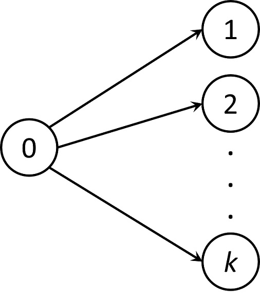
In this document we present how to estimate and test cause specific hazard ratio for the probability of experiencing a certain event at a given time in a competing risks model in R. We focus on the basic model where each subject experiences only one out of k possible events as depicted in the figure below.
As this document aims to provide syntax for estimating and testing cause-specific hazard ratios using Cox’s PH model for competing risks, we assume that readers have working knowledge of a competing risks framework. The Reference below list a few literature for a quick refresher on this topic.
The syntax given here produce results match that produced by the default settings of SAS PROC PHREG (see the companion SAS document). This is usually necessary if validating results from the two software is the objective.
R Package
We use the survival package in this document.
Data used
The bone marrow transplant (BTM) dataset as presented by Guo & So (2018) is used. The dataset has the following variables:
Grouphas three levels, indicating three disease groups.Tis the disease-free survival time in days. A derived variableTYears = T/365.25is used in the analysis.Statushas value 0 ifTis censored; 1 ifTis time to relapse; 2 ifTis time to death.WaitTimeis the waiting time to transplant in days.For illustration, a categorical variable
waitCatis created fromwaitTimeaswaitCat = TRUEifwaitTime > 200, andFALSEotherwise.
bmt <- haven::read_sas(file.path("../data/bmt.sas7bdat")) %>%
  mutate(
    Group = factor(
      Group,
      levels = c(1, 2, 3),
      labels = c('ALL', 'AML-Low Risk', 'AML-High Risk')
    ),
    Status = factor(
      Status,
      levels = c(0, 1, 2),
      labels = c('Censored', 'Relapse', 'Death')
    ),
    TYears = T / 365.25,
    waitCat = (WaitTime > 200),
    ID = row_number()
  )
Estimating and testing the cause specific hazard ratio
Syntax-wise there are two ways to generate the estimates and related outputs using survival::coxph(). They produce essentially the same results except that the global null hypotheses are different.
Syntax 1: All competing events in one go
csh.1 <- survival::coxph(
  survival::Surv(TYears, Status) ~ Group + survival::strata(waitCat),
  data = bmt,
  id = ID,
  ties = 'breslow', ## default is 'efron'
  robust = FALSE ## default is TRUE
)
summary(csh.1)
Call:
survival::coxph(formula = survival::Surv(TYears, Status) ~ Group +
survival::strata(waitCat), data = bmt, ties = "breslow",
robust = FALSE, id = ID)
n= 137, number of events= 83
coef exp(coef) se(coef) z Pr(>|z|)
GroupAML-Low Risk_1:2 -0.9453 0.3886 0.4508 -2.097 0.0360 *
GroupAML-High Risk_1:2 0.6162 1.8519 0.3636 1.695 0.0901 .
GroupAML-Low Risk_1:3 -0.3987 0.6712 0.3946 -1.010 0.3123
GroupAML-High Risk_1:3 0.1273 1.1358 0.4031 0.316 0.7521
---
Signif. codes: 0 '***' 0.001 '**' 0.01 '*' 0.05 '.' 0.1 ' ' 1
exp(coef) exp(-coef) lower .95 upper .95
GroupAML-Low Risk_1:2 0.3886 2.5736 0.1606 0.940
GroupAML-High Risk_1:2 1.8519 0.5400 0.9081 3.777
GroupAML-Low Risk_1:3 0.6712 1.4899 0.3097 1.455
GroupAML-High Risk_1:3 1.1358 0.8804 0.5154 2.503
Concordance= 0.619 (se = 0.031 )
Likelihood ratio test= 17.36 on 4 df, p=0.002
Wald test = 16.13 on 4 df, p=0.003
Score (logrank) test = 17.83 on 4 df, p=0.001In the output, rows with suffix 1:2 are for Status = 2, or Relapse; and 1:3 are for Status = 3, or Death. As usual, censoring must be the lowest level in Status, which in this example is coded 0.
Since both events (Relapse and Death) are model together, the global tests have 4 degrees of freedom, with the null hypothesis that there is no difference among different levels of Group in either Relapse or Death.
Syntax 2: One event at a time
csh.2 <- survival::coxph(
  survival::Surv(TYears, Status == 'Relapse') ~
    Group + survival::strata(waitCat),
  data = bmt,
  id = ID,
  ties = 'breslow', ## default is 'efron'
  robust = FALSE ## default is TRUE
)
summary(csh.2)
Call:
survival::coxph(formula = survival::Surv(TYears, Status == "Relapse") ~
Group + survival::strata(waitCat), data = bmt, ties = "breslow",
robust = FALSE, id = ID)
n= 137, number of events= 42
coef exp(coef) se(coef) z Pr(>|z|)
GroupAML-Low Risk -0.9453 0.3886 0.4508 -2.097 0.0360 *
GroupAML-High Risk 0.6162 1.8519 0.3636 1.695 0.0901 .
---
Signif. codes: 0 '***' 0.001 '**' 0.01 '*' 0.05 '.' 0.1 ' ' 1
exp(coef) exp(-coef) lower .95 upper .95
GroupAML-Low Risk 0.3886 2.574 0.1606 0.940
GroupAML-High Risk 1.8519 0.540 0.9081 3.777
Concordance= 0.672 (se = 0.039 )
Likelihood ratio test= 15.37 on 2 df, p=5e-04
Wald test = 14.16 on 2 df, p=8e-04
Score (logrank) test = 15.83 on 2 df, p=4e-04The results are identical to those labeled with 1:2 in the earlier outputs under Syntax 1 above. However, since only Relapse is modeled, the global tests have only 2 degrees of freedom with the null hypothesis that there is no difference among different levels of Group for Relapse.
Summary
In
survival::coxph()the default method for handling ties isties = 'efron'. To match results with SAS, this needs to be changed toties =breslow`.For multi-state models such as a competing risk analysis,
survival::coxph()by default estimate the standard errors of parameter estimates with a robust sandwich estimator. To match default results with SAS, this needs to be set torobust = FALSE.Due to differences in internal numerical estimation methods of R and SAS, results only match up to the 4th decimal places. However, overall consistency can be established between the two for estimating and testing cause-specific hazard ratio using Cox’s PH model.
NoteSession Info
─ Session info ───────────────────────────────────────────────────────────────
 setting  value
 version  R version 4.5.2 (2025-10-31)
 os       Ubuntu 24.04.3 LTS
 system   x86_64, linux-gnu
 ui       X11
 language (EN)
 collate  en_US.UTF-8
 ctype    en_US.UTF-8
 tz       Europe/London
 date     2026-03-17
 pandoc   3.6.3 @ /home/michael/.positron-server/bin/f3aae65e0a1a11d39226cd884520f49301daef82/quarto/bin/tools/x86_64/ (via rmarkdown)

─ Packages ───────────────────────────────────────────────────────────────────
 package    * version date (UTC) lib source
 cmprsk       2.2-12  2024-05-19 [1] RSPM (R 4.5.0)
 survival   * 3.8-3   2024-12-17 [2] CRAN (R 4.5.2)
 tidycmprsk   1.1.1   2025-11-14 [1] RSPM (R 4.5.0)

 [1] /home/michael/source/personal/CAMIS/renv/library/linux-ubuntu-noble/R-4.5/x86_64-pc-linux-gnu
 [2] /opt/R/4.5.2/lib/R/library

──────────────────────────────────────────────────────────────────────────────
Reference
Guo C and So Y. (2018). “Cause-specific analysis of competing risks using the PHREG procedure.” In Proceedings of the SAS Global Forum 2018 Conference. Cary, NC: SAS Institute Inc. https://support.sas.com/resources/papers/proceedings18/2159-2018.pdf.
Pintilie M. (2006). Competing Risks: A Practical Perspective. Wiley. http://dx.doi.org/10.1002/9780470870709
Therneau T, Crowson C, and Atkinson E. (2024). “Multi-state models and competing risks.” https://cran.r-project.org/web/packages/survival/vignettes/compete.pdf