knitr::include_graphics('../images/cmh/img.png')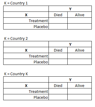
The CMH procedure tests for conditional independence in partial contingency tables for a 2 x 2 x K design. However, it can be generalized to tables of X x Y x K dimensions.
knitr::include_graphics('../images/cmh/img.png')
For the remainder of this document, we adopt the following naming convention when referring to variables of a contingency table:
X = exposure (often the treatment variable)
Y = response (the variable of interest)
K = control/strata (often a potential confounder you want to control for)
The scale of the exposure (X) and response (Y) variables dictate which test statistic is computed for the contingency table. Each test statistic is evaluated on different degrees of freedom (df):
General association statistic (X and Y both nominal) results in (X-1) * (Y-1) dfs
Row mean scores statistic (X is nominal and Y is ordinal) results in X-1 dfs
Nonzero correlation statistic (X and Y both ordinal) results in 1 df
To begin investigating the differences in the SAS and R implementations of the CMH test, we decided to use the CDISC Pilot data set, which is publicly available on the PHUSE Test Data Factory repository. We applied very basic filtering conditions upfront (see below) and this data set served as the basis of the examples to follow.
data <- read.csv("../data/adcibc.csv")
head(data)
X STUDYID SITEID SITEGR1 USUBJID TRTSDT TRTEDT
1 1 CDISCPILOT01 701 701 01-701-1015 2014-01-02 2014-07-02
2 2 CDISCPILOT01 701 701 01-701-1023 2012-08-05 2012-09-01
3 3 CDISCPILOT01 701 701 01-701-1028 2013-07-19 2014-01-14
4 4 CDISCPILOT01 701 701 01-701-1033 2014-03-18 2014-03-31
5 5 CDISCPILOT01 701 701 01-701-1034 2014-07-01 2014-12-30
6 6 CDISCPILOT01 701 701 01-701-1047 2013-02-12 2013-03-09
TRTP TRTPN AGE AGEGR1 AGEGR1N RACE RACEN SEX ITTFL EFFFL
1 Placebo 0 63 <65 1 WHITE 1 F Y Y
2 Placebo 0 64 <65 1 WHITE 1 M Y Y
3 Xanomeline High Dose 81 71 65-80 2 WHITE 1 M Y Y
4 Xanomeline Low Dose 54 74 65-80 2 WHITE 1 M Y Y
5 Xanomeline High Dose 81 77 65-80 2 WHITE 1 F Y Y
6 Placebo 0 85 >80 3 WHITE 1 F Y Y
COMP24FL AVISIT AVISITN VISIT VISITNUM ADY ADT PARAMCD
1 Y Week 8 8 WEEK 8 8 63 2014-03-05 CIBICVAL
2 N Week 8 8 WEEK 4 5 29 2012-09-02 CIBICVAL
3 Y Week 8 8 WEEK 8 8 54 2013-09-10 CIBICVAL
4 N Week 8 8 WEEK 4 5 28 2014-04-14 CIBICVAL
5 Y Week 8 8 WEEK 8 8 57 2014-08-26 CIBICVAL
6 N Week 8 8 AMBUL ECG REMOVAL 6 46 2013-03-29 CIBICVAL
PARAM PARAMN AVAL ANL01FL DTYPE AWRANGE AWTARGET AWTDIFF AWLO AWHI AWU
1 CIBIC Score 1 4 Y NA 2-84 56 7 2 84 DAYS
2 CIBIC Score 1 3 Y NA 2-84 56 27 2 84 DAYS
3 CIBIC Score 1 4 Y NA 2-84 56 2 2 84 DAYS
4 CIBIC Score 1 4 Y NA 2-84 56 28 2 84 DAYS
5 CIBIC Score 1 4 Y NA 2-84 56 1 2 84 DAYS
6 CIBIC Score 1 4 Y NA 2-84 56 10 2 84 DAYS
QSSEQ
1 6001
2 6001
3 6001
4 6001
5 6001
6 6001In order to follow a systematic approach to testing, and to cover variations in the CMH test, we considered the traditional 2 x 2 x K design as well as scenarios where the generalized CMH test is employed (e.g. 5 x 3 x 3).
We present 6 test scenarios, some of which have sparse data.
| Number | Schema (X x Y x K) | Variables | Relevant Test | Description |
|---|---|---|---|---|
| 1 | 2x2x2 | X = TRTP, Y = SEX, K = AGEGR1 | General Association | TRTP and AGEGR1 were limited to two categories (removing the low dose and >80 year group), overall the the groups were rather balanced |
| 2 | 3x2x3 | X = TRTP, Y = SEX, K = AGEGR1 | General Association | TRTP and AGEGR1 each have 3 levels, SEX has 2 levels, overall the the groups were rather balanced |
| 3 | 3x2x3 | X = TRTP, Y = SEX, K = RACE | General Association | One stratum of RACE has only n=1 |
| 6 | 2x5x2 | X = TRTP, Y = AVAL, K = SEX | Row Means | Compare Row Means results because Y is ordinal |
| 9 | 3x5x17 | X = TRTP, Y = AVAL, K = SITEID | Row Means | SITEID has many strata and provokes sparse groups; AVAL is ordinal, therefore row means statistic applies here |
| 10 | 5x3x3 | X = AVAL, Y = AGEGR1N, K = TRTP | Correlation | X and Y are ordinal variables and therefore the correlation statistics can be used |
sas_results <- tribble(
  ~Scenario, ~Test, ~Chisq, ~Df, ~Prob,
  1L ,"Correlation",         0.2166, 1, 0.6417,
  1L ,"Row Means",           0.2166, 1, 0.6417,
  1L ,"General Association", 0.2166, 1, 0.6417,

  2L ,"Correlation",         0.0009, 1, 0.9765,
  2L ,"Row Means",           2.4820, 1, 0.2891,
  2L ,"General Association", 2.4820, 1, 0.2891,

  3L ,"Correlation",         0.0028, 1, 0.9579,
  3L ,"Row Means",           2.3861, 2, 0.3033,
  3L ,"General Association", 2.3861, 2, 0.3033,

  6L ,"Correlation",         1.7487, 1, 0.1860,
  6L ,"Row Means",           1.7487, 1, 0.1860,
  6L ,"General Association", 8.0534, 4, 0.0896,

  9L ,"Correlation",         0.0854, 1, 0.7701,
  9L ,"Row Means",           2.4763, 2, 0.2899,
  9L ,"General Association", 7.0339, 8, 0.5330,

  10L ,"Correlation",        1.6621, 1, 0.1973,
  10L ,"Row Means",          2.2980, 4, 0.6811,
  10L ,"General Association",5.7305, 8, 0.6774
) |>
mutate(lang = "SAS")library(vcdExtra)Loading required package: vcdLoading required package: gridLoading required package: gnmRegistered S3 method overwritten by 'vcdExtra':
method from
print.Kappa vcd
Attaching package: 'vcdExtra'The following object is masked from 'package:vcd':
woolf_testdata2 <- data |>
filter(TRTPN != "54" & AGEGR1 != ">80")
s1 <- vcdExtra::CMHtest(
Freq ~ TRTP + SEX | AGEGR1,
data = data2,
overall = TRUE
)$ALL$table
s2 <- vcdExtra::CMHtest(
Freq ~ TRTP + SEX | AGEGR1,
data = data,
overall = TRUE
)$ALL$table
s3 <- vcdExtra::CMHtest(
Freq ~ TRTP + SEX | RACE,
data = data,
overall = TRUE
)$ALL$table
s6 <- vcdExtra::CMHtest(
Freq ~ TRTP + AVAL | SEX,
data = data2,
overall = TRUE
)$ALL$table
## Unable to run: For large sparse table (many strata) CMHTest will occasionally throw an error in solve.default(AVA) because of singularity
# s9 <- vcdExtra::CMHtest(
# Freq ~ TRTP + AVAL | SITEID,
# data = data, overall = TRUE
# )$ALL$table
s10 <- vcdExtra::CMHtest(
Freq ~ AVAL + AGEGR1N | TRTP,
data = data,
overall = TRUE
)$ALL$table
# Summarize the results
r_results <- list(s1, s2, s3, s6, s10) |>
map(function(x) {
as_tibble(x) |>
mutate(across(everything(), unlist), Test = rownames(x))
}) |>
reduce(bind_rows) |>
mutate(
Scenario = rep(c(1, 2, 3, 6, 10), each = 4),
Test = case_when(
Test == "cor" ~ "Correlation",
Test == "rmeans" ~ "Row Means",
Test == "general" ~ "General Association"
),
lang = "R"
) |>
filter(!is.na(Test))As can be seen, there are 2 scenarios where vcdExtra in R does not provide any results:
library(gt)

bind_rows(sas_results, r_results) |>
  arrange(Scenario) |>
  pivot_wider(names_from = lang, values_from = c("Chisq", "Df", "Prob")) |>
  gt(
    groupname_col = "Scenario"
  ) |>
  tab_spanner(
    label = "Chi-Square",
    columns = starts_with("Chisq")
  ) |>
  tab_spanner(
    label = "df",
    columns = starts_with("Df")
  ) |>
  tab_spanner(
    label = "p-value",
    columns = starts_with("Prob")
  ) |>
  cols_label(
    Chisq_SAS = "SAS",
    Chisq_R = "R",
    Df_SAS = "SAS",
    Df_R = "R",
    Prob_SAS = "SAS",
    Prob_R = "R"
  ) |>
  tab_options(row_group.as_column = TRUE) |>
  tab_footnote(
    footnote = md(
      "**Reason for NaN in scenario 3**: Stratum k = AMERICAN INDIAN OR ALASKA NATIVE has n=1."
    ),
    cells_row_groups(groups = "3"),
    placement = "right"
  ) |>
  tab_footnote(
    footnote = md(
      "**Reason for in scenario 9:** For large sparse table (many strata) CMHTest will throw an error in solve.default(AVA) because of singularity"
    ),
    cells_row_groups(groups = "9"),
    placement = "right"
  ) |>
opt_footnote_marks(marks = "standard")| Test |
Chi-Square
|
df
|
p-value
|
||||
|---|---|---|---|---|---|---|---|
| SAS | R | SAS | R | SAS | R | ||
| 1 | Correlation | 0.2166 | 0.2165549886 | 1 | 1 | 0.6417 | 0.64167748 |
| Row Means | 0.2166 | 0.2165549886 | 1 | 1 | 0.6417 | 0.64167748 | |
| General Association | 0.2166 | 0.2165549886 | 1 | 1 | 0.6417 | 0.64167748 | |
| 2 | Correlation | 0.0009 | 0.0008689711 | 1 | 1 | 0.9765 | 0.97648311 |
| Row Means | 2.4820 | 2.4820278527 | 1 | 2 | 0.2891 | 0.28909095 | |
| General Association | 2.4820 | 2.4820278527 | 1 | 2 | 0.2891 | 0.28909095 | |
| 3* | Correlation | 0.0028 | 0.0027871297 | 1 | 1 | 0.9579 | 0.95789662 |
| Row Means | 2.3861 | 2.3860698467 | 2 | 2 | 0.3033 | 0.30329938 | |
| General Association | 2.3861 | 2.3860698467 | 2 | 2 | 0.3033 | 0.30329938 | |
| 6 | Correlation | 1.7487 | 1.7487003723 | 1 | 1 | 0.1860 | 0.18604020 |
| Row Means | 1.7487 | 1.7487003723 | 1 | 1 | 0.1860 | 0.18604020 | |
| General Association | 8.0534 | 8.0533878514 | 4 | 4 | 0.0896 | 0.08964199 | |
| 9† | Correlation | 0.0854 | NA | 1 | NA | 0.7701 | NA |
| Row Means | 2.4763 | NA | 2 | NA | 0.2899 | NA | |
| General Association | 7.0339 | NA | 8 | NA | 0.5330 | NA | |
| 10 | Correlation | 1.6621 | 1.6620500937 | 1 | 1 | 0.1973 | 0.19732675 |
| Row Means | 2.2980 | 2.2980213984 | 4 | 4 | 0.6811 | 0.68112931 | |
| General Association | 5.7305 | 5.7305381934 | 8 | 8 | 0.6774 | 0.67738613 | |
| * Reason for NaN in scenario 3: Stratum k = AMERICAN INDIAN OR ALASKA NATIVE has n=1. | |||||||
| † Reason for in scenario 9: For large sparse table (many strata) CMHTest will throw an error in solve.default(AVA) because of singularity | |||||||
Having explored the available R packages to calculate the CMH statistics, the base stats::mantelhaen.test() function can be recommended for the classic CMH test in the 2 x 2 x K scenarios. The vcdExtra package shows matching results with SAS, however in cases with sparse data the vcdExtra package will not provide results.
The base stats::mantelhaen.test() function does return results in cases of sparse data (required n > 1 in each strata).
Accessible Summary: https://online.stat.psu.edu/stat504/lesson/4/4.4
An Introduction to Categorical Data Analysis 2nd Edition (Agresti): http://users.stat.ufl.edu/~aa/
SAS documentation (Specification): https://documentation.sas.com/doc/en/pgmsascdc/9.4_3.3/statug/statug_freq_examples07.html
SAS documentation (Theoretical Basis + Formulas): https://documentation.sas.com/doc/en/pgmsascdc/9.4_3.5/procstat/procstat_freq_details92.html
Original Paper 1: https://doi.org/10.2307%2F3001616
Original Paper 2: https://doi.org/10.1093/jnci/22.4.719