Group Sequential Design in Survival Endpoints Using SAS
Introduction
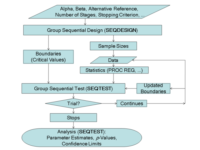
PROC SEQDESIGN1 can be used for sample size calculations for group sequential design (GSD). SAS provides a flowchart2 which summarizes the steps in a typical group sequential trial and the relevant SAS procedures. Here we focus on a GSD applied for time-to-event endpoints.
Log-Rank Test for Two Survival Distributions
This example illustrates sample size computation for survival data with the same setting in another R example:
A GSD will be utilized for progression-free survival (PFS). PFS will be tested at one interim analysis (IA) at 75% information fraction for both efficacy and non-binding futility. A Lan-DeMets O’Brien-Fleming-type (LD-OBF) spending function will be used for efficacy testing, and a Hwang-Shih-Decani (HSD) spending function (as known as gamma cumulative spending function) with \(\gamma = -10\) will be used for futility. In the GSD, \(\alpha\) is one-sided at 0.025, \(\beta\) is 0.05, the accrual period is 24 months, and the follow-up period is 10 months. As described in the R example, the dropout rates are 0.2 by month 12 for the both group; that is, the dropout times follow the exponential distribution with the parameter \(\lambda = -\ln(1-0.2)/12 = 0.0185953\).
The SAS code is shown below:
PROC SEQDESIGN;
DESIGN NSTAGES=2
INFO=CUM(0.75 1.0)
ALT=UPPER
ALPHA=0.0125
BETA=0.05
METHOD(ALPHA)=ERRFUNCOBF
METHOD(BETA)=ERRFUNCGAMMA(GAMMA=-10)
STOP=BOTH(BETABOUNDARY=NONBINDING);
SAMPLESIZE MODEL=TWOSAMPLESURVIVAL(
NULLMEDSURVTIME=9.4
HAZARDRATIO=0.6
ACCTIME=24
FOLTIME=10
LOSS=EXP(HAZARD=0.0185953)
WEIGHT=1);
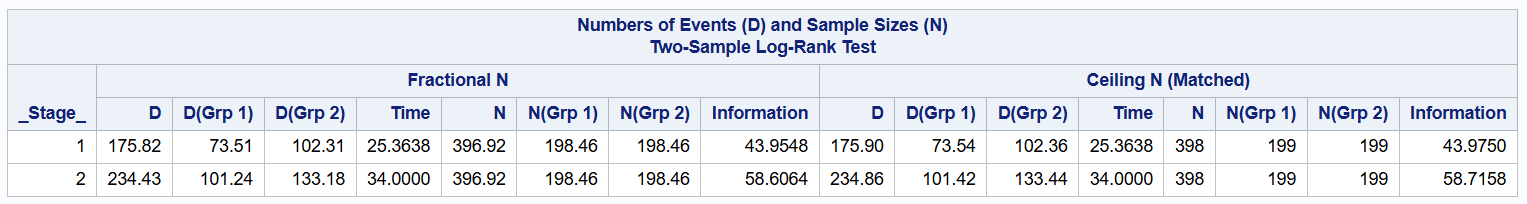
RUN;As shown below, a total sample size of 398 is recommended, which equates to 199 in each group.