Accelerated Failure Time (AFT) - SAS
INTRODUCTION
Accelerated Failure Time (AFT) models are parametric models, where the effect of an explanatory variable is to speed up or slow down the survival time.
Consider two groups: Group C (control group) and Group T (new treatment), under an AFT formulation, the survival functions of the two groups are related through a time-scaling factor ϕ, comparing T vs C:
ϕ <1: the event happens earlier in group T a than in group C , an acceleration of time to event (survival time decreases in new treatment group).
ϕ =1: No effect on survival time.
ϕ >1: the event happens later in group T a than in group C , a deceleration of time to event (survival time increases in new treatment group).
See further maths information in the R section: https://psiaims.github.io/CAMIS/R/Accelerated_Failure_time_model.html
In SAS, several distributions that can be fitted in PROC LIFEREG, the following sections explore the most commonly used ones: Log-Normal, Log-Logistic and Weibull (by default).
AFT with”Weibull” (Default)
Data
For consistency with the R example, the ovarian dataset from the R survival package [1] is used for the Weibull model example. This dataset contains survival data from a randomized trial comparing two treatments for ovarian cancer. It includes 26 observations and 6 variables describing patient characteristics, treatment assignment, and survival outcomes:
futime: survival or censoring time
fustat: censoring status (1=deceased, 0 = alive)
age: in years
resid.ds: residual disease present (1=no, 2=yes)
rx: treatment group (1 = standard treatment, 2 = experimental treatment)
ecog.ps: ECOG performance status
In this example, the variables time to event is analyzed including the variables age, residual disease present and treatment group.
Code
The MODEL statement in PROC LIFEREG follows a syntax similar to that of PROC LIFETEST, where the time-to-event variable is specified together with the censoring indicator using the form time*status(x), with xindicating the value corresponding to censored observations. In this example, a Weibull distribution is assumed (DIST=weibull), which is also the default.
The acceleration factor can be exponentiating the estimated regression coefficients. The exponentiation can be done by using the estimate statement with the exp option; or storing the coefficients in a dataset, and applying the exponential transformation in a data step. Additionally, with the estimate statement allows to obtain results for different comparisons. Also, survival time predicted by the model, can be stored in a dataset by using output out. The following example computes the AR using both approaches.
proc lifereg data=ovarian outest=estimates;

  * Define class variables;
  class rx resid_ds;

  *Define model and distribution;
  model futime*fustat(0)=age resid_ds rx/dist=weibull;

  * Get acceleration factor using estimate;
  estimate 'age'                    age 1   /exp cl;
  estimate 'resid_ds (1 vs 2)' resid_ds 1 -1/exp cl;
  estimate  'rx (1 vs 2)'           rx  1 -1/exp cl;  /* Comparing 1 vs 2*/
  estimate  'rx (2 vs 1)'           rx -1  1/exp cl;  /* Comparing 2 vs 1*/

  output out=pred_wei_SAS predicted=pred; /*Predicted time*/
  ods output ParameterEstimates = coeff;

 run;
data acf;
set coeff;
label af='Acceleration Factor (AF)'
lowercl='AF Lower Limit'
uppercl='AF Lower Limit';
af=exp(estimate);
lowercl=exp(lowercl);
uppercl=exp(uppercl);
if (level1 ne '' and estimate=0) or parameter in ('Scale' 'Weibull Shape' 'Intercept') then delete;
run;
proc print data=acf noobs label;
title 'Acceleration factor';
var parameter level1 af lowercl uppercl;
format af lowercl uppercl 9.4;
run;
Interpretation
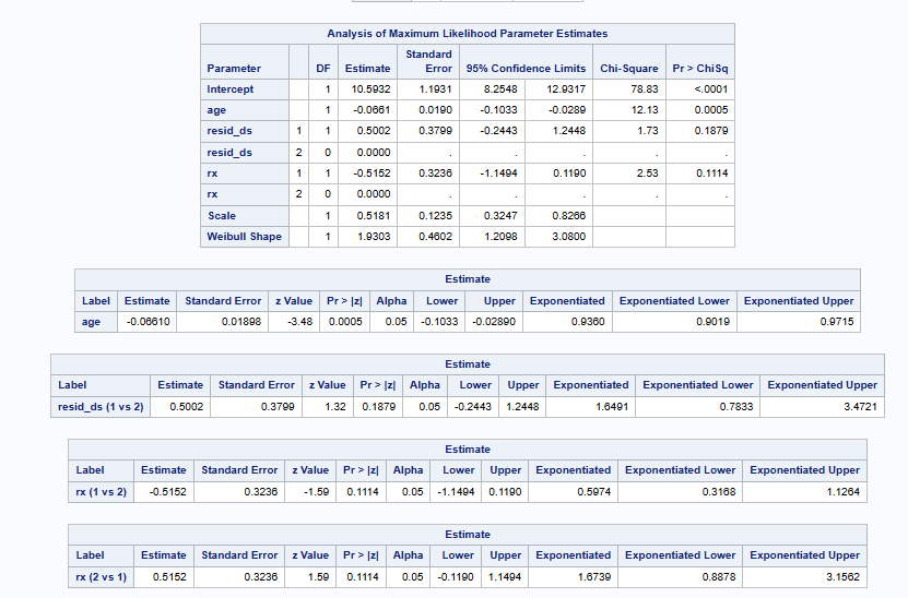
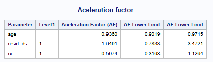
For age, an acceleration factor ϕ = 0.9360 indicates that events occur more quickly (accelerated failure) so for each 1-unit increase in age, the time to event is reduced by approximately 6.4%.
For residual disease status (1: No vs 2: Yes), an acceleration factor of ϕ =1.6491 indicates that subjects without residual disease have longer survival times compared with those with residual disease. In other words, the time to event is approximately 64.9% longer for patients with no residual disease.
For treatment, The acceleration factor for treatment is assessed in two directions (1 vs 2 and 2 vs 1):
1: standard vs 2 experimental treatment: An acceleration factor of ϕ=0.5974 indicates that the standard treatment is associated with shorter survival times, with the time to event being approximately 40.3% shorter compared to the experimental treatment.
2: experimental vs 1 standard treatment: Conversely, when expressed in the reverse direction, an acceleration factor of ϕ=1.6739 indicates that the experimental treatment is associated with longer survival times, with the time to event being approximately 67.4% longer compared to the standard treatment.
AFT using Log-Normal Distribution
Data
For consistency with the R example, the same lung dataset from the R survival package is used in this example. This dataset contains the following variables:
inst: Institution code
time: Survival time in days
status: censoring status (1=censored, 2=dead)
age: Age in years
sex: (1 = male, 2 = female)
ph.ecog: ECOG performance score as rated by the physician.
ph.karno: Karnofsky performance score (bad=0-good=100) rated by physician
pat.karno: Karnofsky performance score as rated by patient
meal.cal: Calories consumed at meals
wt.loss: Weight loss in last six months (pounds)
In this example, age, sex, and ECOG are included as covariates. Age and ECOG are modeled as continuous variables, while sex is treated as categorical. Since ECOG is not stored numerically, it is converted to a numeric variable in a data step for non-missing observations.
data lung1;
 set lung;
 if ph_ecog NE 'NA' then ph_ecogn=input(ph_ecog, 1.);
run;
Code
In this example, a log-normal distribution is assumed (DIST=LNORMAL).
proc lifereg data=lung1;
  class sex;

  model time*status(1)=age sex ph_ecogN/dist=lnormal;

  * Get acceleration factor using estimate;
  estimate 'age'        age 1/exp cl;
  estimate 'sex 2 vs 1' sex 1 -1 / exp cl;
  estimate 'ph_ecogN'  ph_ecogN 1/exp cl;

  output out=pred_wei_SAS predicted=pred; /*Predicted time*/
  ods output ParameterEstimates = coeff;
run;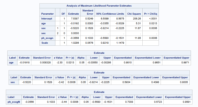
 /* Get acceleration factor in a data step */
 data acf;
   set coeff;
   af=exp(estimate);
   lowercl=exp(estimate);
   uppercl=exp(estimate);
   format _all_ 8.4;
 run;

 proc print data=acf noobs;
  title 'Acceleration factor';
 run;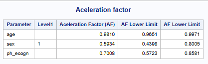
AFT with log-logistic
Data
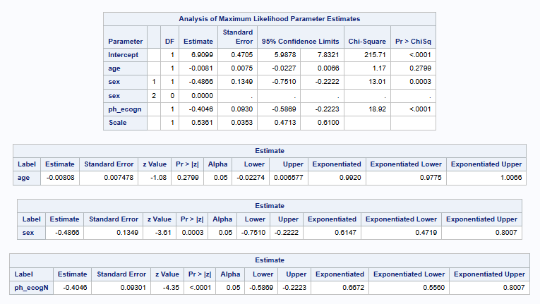
In this example, the same dataset and set of covariates are retained as in the log-normal case, with the only modification being the assumption of a log-logistic distribution (DIST=LLOGISTIC).
Code
proc lifereg data=lung1;
  class sex;

  model time*status(1)=age sex ph_ecogN/dist=llogistic;

  * Get acceleration factor using estimate;
  estimate 'age'        age 1/exp cl;
  estimate 'sex 2 vs 1' sex 1 -1 / exp cl;
  estimate 'ph_ecogN'  ph_ecogN 1/exp cl;

  * Store results in datasets;
  ods output ParameterEstimates = coeff estimates=estimate;
run;
 /* Get acceleration factor in a data step */
 data acf;
   set estimates;
   af=exp(estimate);
   lowercl=exp(estimate);
   uppercl=exp(estimate);
   format _all_ 8.4;
 run;

 proc print data=acf noobs;
  title 'Acceleration factor';
 run;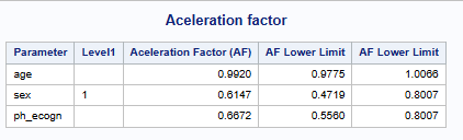
RERERENCES
[1] Therneau TM. A Package for Survival Analysis in R (survival vignette).
[2] SAS Institute Inc. SAS/STAT® User’s Guide: The LIFEREG Procedure.