Independent Two-Sample t-test
Data Used
The following data was used in this example.
data d1;
    length trt_grp $ 9;
    input trt_grp $ WtGain @@;
    datalines;
placebo    94 placebo    12 placebo    26 placebo    89
placebo    88 placebo    96 placebo    85 placebo   130
placebo    75 placebo    54 placebo   112 placebo    69
placebo   104 placebo    95 placebo    53 placebo    21
treatment  45 treatment  62 treatment  96 treatment 128
treatment 120 treatment  99 treatment  28 treatment  50
treatment 109 treatment 115 treatment  39 treatment  96
treatment  87 treatment 100 treatment  76 treatment  80
;
run;
Independent Two-Sample t-test in SAS
The null hypothesis of the Independent Samples t-test is, the means for the two populations are equal.
In SAS the following code was used to test the mean comparison (mean of Weight Gain) of two independent treatment groups (Treatment and Placebo). Both the Student’s t-test and Welch’s t-test (the Satterthwaite approximation is used to calculate the effective degrees of freedom and variance) in the same call.
For this example, we’re testing the significant difference in mean of Weight gain (WtGain) between treatment and placebo (trt_grp) using PROC TTEST procedure in SAS.
proc ttest data=d1;
    class trt_grp;
    var WtGain;
run;
Output:
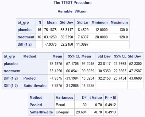
Figure 1: Test results for independent t-test using PROC TTEST in SASHere the t-value is –0.70, degrees of freedom is 30 and P value is 0.4912 which is greater than 0.05, so we accept the null hypothesis that there is no evidence of a significant difference between the means of treatment groups. The mean in placebo group is 75.1875 and mean in Treatment group is 83.1250. The mean difference the treatment groups (Treatment-Placebo) is –7.9375 and the 95% CI for the mean difference is [–31.1984, 15.3234]. The 95% confidence interval includes a treatment difference of 0, which supports the conclusion that the data fail to provide any evidence of a difference between the treatment groups.
Model Checking
Note: Before entering straight into the t-test we need to check whether the assumptions (like the equality of variance, the observations should be independent, observations should be normally distributed) are met or not. If normality is not satisfied, we may consider using a suitable non-parametric test.
- Normality: You can check for data to be normally distributed by plotting a histogram of the data by treatment. Alternatively, you can use the Shapiro-Wilk test or the Kolmogorov-Smirnov test. If the test is <0.05 and your sample is quite small then this suggests you should not use the t-test. However, if your sample in each treatment group is large (say >30 in each group), then you do not need to rely so heavily on the assumption that the data have an underlying normal distribution in order to apply the two-sample t-test. This is where plotting the data using histograms can help to support investigation into the normality assumption. We have checked the normality of the observations using the code below. Here for both the treatment groups we have P value greater than 0.05 (Shapiro-Wilk test is used), therefore the normality assumption is there for our data.
proc univariate data=d1 normal;
    qqplot WtGain;
    by trt_grp;
run;
Output:
Figure 2: The results of normality test for Treatment group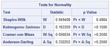
Figure 3: The results of normality test for Placebo group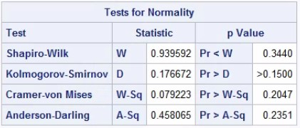
- Homogeneity of variance (or Equality of variance): Homogeniety of variance will be tested by default in PROC TTEST itself by Folded F-test. In our case the P values is 0.6981 which is greater than 0.05. So we accept the null hypothesis of F-test, i.e. variances are same. Then we will consider the pooled method for t-test. If the F test is statistically significant (p<0.05), then the pooled t-test may give erroneous results. In this instance, if it is believed that the population variances may truly differ, then the Satterthwaite (unequal variances) analysis results should be used. These are provided in the SAS output alongside the Pooled results as default.
Output:
Figure 4: Folded F-test result in PROC TTEST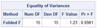
Example with unequal variances
For this example, it is important to use the Welch’s t-test (the Satterthwaite approximation is used to calculate the effective degrees of freedom and variance) results.
data d2;
    length trt_grp $ 9;
    input trt_grp $ WtGain @@;
    datalines;
placebo    14 placebo    15 placebo    15 placebo    15
placebo    16 placebo    18 placebo    22 placebo    23
placebo    24 placebo    25 placebo    25
treatment  10 treatment  12 treatment  14 treatment  15
treatment  18 treatment  22 treatment  24 treatment  27
treatment  31 treatment  33 treatment  34 treatment  34
treatment  34
;
run;

proc ttest data=d2;
    class trt_grp;
    var WtGain;
run;
Output:
Figure 1: Test results for independent t-test using PROC TTEST in SAS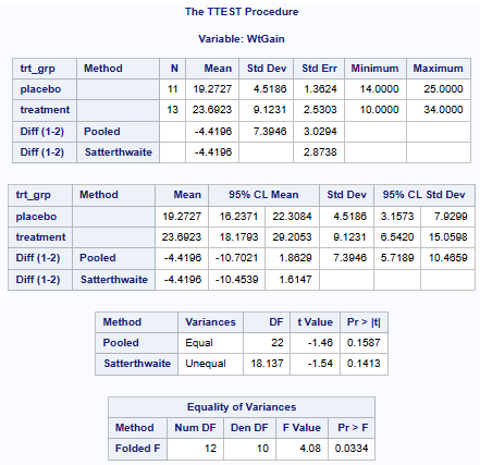
Lognormal Data
The SAS two-sample t-test also supports lognormal analysis for a two-sample t-test.
Code
Using the same d1 dataset as above, we will set the “DIST” option to “lognormal” and specify a CLASS variable to perform this analysis:
proc ttest data=d1 dist=lognormal;
  class trt_grp;
  var wtgain;
run;
Output:
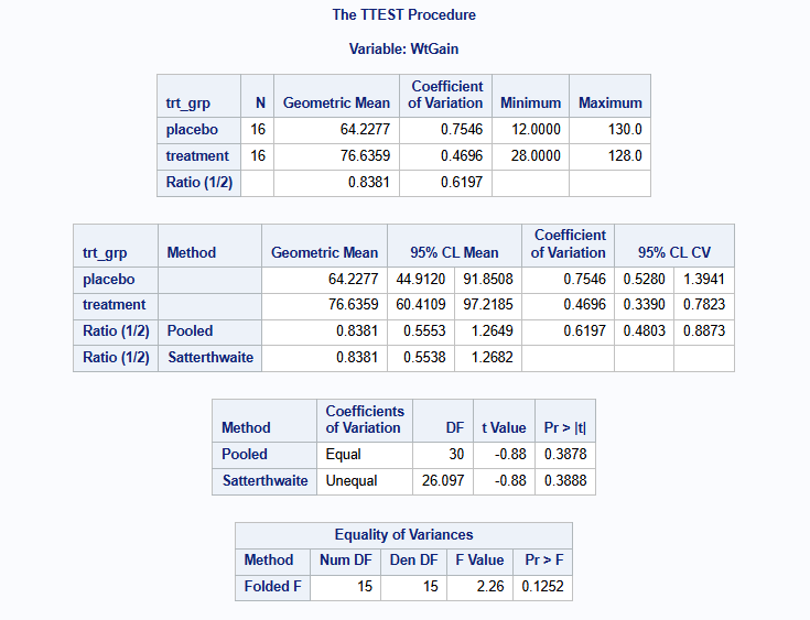
As can be seen in the figure above, the lognormal variation of the two-sample t-test provides results for geometric mean by group, geometric mean ratio, coefficient of variation, and 95% confidence limits for the ratio and coefficient of variation.