# General libraries
library(mice)
library(dplyr)
library(tidyr)
library(gt)
library(labelled)
library(purrr)
library(ggplot2)
library(gridExtra)

# Methodology specific libraries
library(emmeans)
library(mmrm)
library(rstan)
library(rbmi)

# Paralleisation libraries
library(future)
library(furrr)
library(parallelly)R Tipping Point (Delta Adjustment): Continuous Data
Tipping Point / Delta Adjustment
Setup
Random seed
set.seed(12345)Reference-based multiple imputation (rbmi)
Methodology introduction
The concept of delta adjustment and tipping point analysis builds on the framework of reference-based multiple imputation (rbmi) as seen on its respective CAMIS webpage. The use of the rbmi package in R (Gower-Page et al. 2022) for the following standard and reference-based multiple imputation approaches are introduced there:
Missing At Random (MAR)
Jump to Reference (JR)
Copy Reference (CR)
Copy Increment from Reference (CIR)
Please make sure to familiarize yourself with these functionalities of the rbmi package before checking this tutorial. The outline of this page generally follows the rbmi advanced functionality vignette.
Data
The same publicly available dataset from an antidepressant clinical trial that was used to illustrate rbmi is again used for this tutorial. This dataset is also used in the rbmi quickstart vignette.
The relevant endpoint for the antidepressant trial was assessed using the Hamilton 17-item depression rating scale (HAMD17), which was measured at baseline and subsequently at weeks 1, 2, 3, 4 and 6 (visits 4-7). Study drug discontinuation occurred in 24% (20/84) of subjects in the active drug group, compared to 26% (23/88) of subjects in the placebo group. Importantly, all data after study drug discontinuation are missing and there is a single intermittent missing observation.
data("antidepressant_data")

dat <- antidepressant_data |>
  dplyr::select(
    PATIENT,
    GENDER,
    THERAPY,
    RELDAYS,
    VISIT,
    BASVAL,
    HAMDTL17,
    CHANGE
  ) |>
  dplyr::mutate(THERAPY = factor(THERAPY, levels = c("PLACEBO", "DRUG"))) |>
  labelled::remove_labels()

gt(head(dat, n = 10))| PATIENT | GENDER | THERAPY | RELDAYS | VISIT | BASVAL | HAMDTL17 | CHANGE |
|---|---|---|---|---|---|---|---|
| 1503 | F | DRUG | 7 | 4 | 32 | 21 | -11 |
| 1503 | F | DRUG | 14 | 5 | 32 | 20 | -12 |
| 1503 | F | DRUG | 28 | 6 | 32 | 19 | -13 |
| 1503 | F | DRUG | 42 | 7 | 32 | 17 | -15 |
| 1507 | F | PLACEBO | 7 | 4 | 14 | 11 | -3 |
| 1507 | F | PLACEBO | 15 | 5 | 14 | 14 | 0 |
| 1507 | F | PLACEBO | 29 | 6 | 14 | 9 | -5 |
| 1507 | F | PLACEBO | 42 | 7 | 14 | 5 | -9 |
| 1509 | F | DRUG | 7 | 4 | 21 | 20 | -1 |
| 1509 | F | DRUG | 14 | 5 | 21 | 18 | -3 |
The number of patients per visit and treatment group are:
dat |>
  dplyr::summarise(N = n(), .by = c(VISIT, THERAPY))
# A tibble: 8 × 3
VISIT THERAPY N
<fct> <fct> <int>
1 4 DRUG 84
2 5 DRUG 77
3 6 DRUG 73
4 7 DRUG 64
5 4 PLACEBO 88
6 5 PLACEBO 81
7 6 PLACEBO 76
8 7 PLACEBO 65The mean change from baseline of the HAMD17 endpoint per visit and treatment group using only the complete cases are:
dat |>
  dplyr::summarise(N = n(), MEAN = mean(CHANGE), .by = c(VISIT, THERAPY))
# A tibble: 8 × 4
VISIT THERAPY N MEAN
<fct> <fct> <int> <dbl>
1 4 DRUG 84 -1.82
2 5 DRUG 77 -4.71
3 6 DRUG 73 -6.79
4 7 DRUG 64 -8.34
5 4 PLACEBO 88 -1.51
6 5 PLACEBO 81 -2.70
7 6 PLACEBO 76 -4.07
8 7 PLACEBO 65 -5.14The missingness pattern is:
dat_wide = dat |>
  dplyr::select(PATIENT, VISIT, CHANGE) |>
  pivot_wider(
    id_cols = PATIENT,
    names_from = VISIT,
    names_prefix = "VISIT_",
    values_from = CHANGE
  )

dat_wide |>
  dplyr::select(starts_with("VISIT_")) |>
  mice::md.pattern(plot = TRUE, rotate.names = TRUE)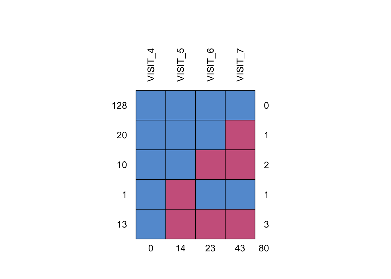
    VISIT_4 VISIT_5 VISIT_6 VISIT_7
128       1       1       1       1  0
20        1       1       1       0  1
10        1       1       0       0  2
1         1       0       1       1  1
13        1       0       0       0  3
          0      14      23      43 80
There is a single patient with an intermittent missing observation at visit 5, which is patient 3618. Special considerations need to be taken when applying delta adjustments to intermittent missing observations like this one (more on this later).
dat_expand <- rbmi::expand_locf(
  dat,
  PATIENT = levels(dat$PATIENT),
  VISIT = levels(dat$VISIT),
  vars = c("BASVAL", "THERAPY", "GENDER"),
  group = c("PATIENT"),
  order = c("PATIENT", "VISIT")
)

dat_expand |>
  dplyr::filter(PATIENT == "3618") |>
gt()| PATIENT | GENDER | THERAPY | RELDAYS | VISIT | BASVAL | HAMDTL17 | CHANGE |
|---|---|---|---|---|---|---|---|
| 3618 | M | DRUG | 8 | 4 | 8 | 15 | 7 |
| 3618 | M | DRUG | NA | 5 | 8 | NA | NA |
| 3618 | M | DRUG | 28 | 6 | 8 | 14 | 6 |
| 3618 | M | DRUG | 42 | 7 | 8 | 10 | 2 |
Preparation
This tutorial will focus on tipping point analysis and delta adjustment. We assume the user used the rbmi package to create an imputation object called imputeObj (see CAMIS webpage).
Tipping point analysis and delta adjustment
Methodology introduction
When analyses for endpoints are performed under MAR or MNAR assumptions for missing data, it is important to perform sensitivity analyses to assess the impact of deviations from these assumptions. Tipping point analysis (or delta adjustment method) is an example of a sensitivity analysis that can be used to assess the robustness of a clinical trial when its result is based on imputed missing data.
Generally, tipping point analysis explores the influence of missingness on the overall conclusion of the treatment difference by shifting imputed missing values in the treatment group towards the reference group until the result becomes non-significant. The tipping point is the minimum shift needed to make the result non-significant. If the minimum shift needed to make the result non-significant is implausible, then greater confidence in the primary results can be inferred.
Tipping point analysis generally happens by adjusting imputing values by so-called delta values. The observed tipping point is the minimum delta needed to make the result non-significant. Mostly a range of delta values is explored and only imputed values from the active treatment group are adjusted by the delta value. However, delta adjustments in the control group are possible as well. Naturally, the range of acceptable values for delta should be agreed a priori, before taking this approach.
For an extensive discussion on delta adjustment methods, we refer to Cro et al. 2020.
Simple delta adjustments
Generate delta’s
In the rbmi package, the delta argument of the analyse() function allows users to adjust the imputed datasets prior to the analysis stage. This delta argument requires a data frame created by delta_template(), which includes a column called delta that specifies the delta values to be added.
By default, delta_template() will set delta to 0 for all observations.
# delta template
dat_delta_0 <- delta_template(imputations = imputeObj)


dat_delta_0 |>
  dplyr::filter(PATIENT %in% c("1513", "1514")) |>
  head(8) |>
gt()| PATIENT | VISIT | THERAPY | is_mar | is_missing | is_post_ice | strategy | delta |
|---|---|---|---|---|---|---|---|
| 1513 | 4 | DRUG | TRUE | FALSE | FALSE | NA | 0 |
| 1513 | 5 | DRUG | TRUE | TRUE | TRUE | MAR | 0 |
| 1513 | 6 | DRUG | TRUE | TRUE | TRUE | MAR | 0 |
| 1513 | 7 | DRUG | TRUE | TRUE | TRUE | MAR | 0 |
| 1514 | 4 | PLACEBO | TRUE | FALSE | FALSE | NA | 0 |
| 1514 | 5 | PLACEBO | TRUE | TRUE | TRUE | MAR | 0 |
| 1514 | 6 | PLACEBO | TRUE | TRUE | TRUE | MAR | 0 |
| 1514 | 7 | PLACEBO | TRUE | TRUE | TRUE | MAR | 0 |
You can add the delta values to the outcome variable (CHANGE) of one of the imputed datasets by using the apply_delta() function. Of course, nothing is changed here as delta = 0.
imputed_dfs = rbmi::extract_imputed_dfs(imputeObj)
MI_10 = imputed_dfs[[10]]
MI_10$PATIENT2 = MI_10$PATIENT
MI_10$PATIENT = dat_expand$PATIENT
# imputed dataset
gt(MI_10 |> dplyr::filter(PATIENT %in% c("1513", "1514")) |> head(8))| PATIENT | GENDER | THERAPY | RELDAYS | VISIT | BASVAL | HAMDTL17 | CHANGE | PATIENT2 |
|---|---|---|---|---|---|---|---|---|
| 1513 | M | DRUG | 7 | 4 | 19 | 24 | 5.000000 | new_pt_5 |
| 1513 | M | DRUG | NA | 5 | 19 | NA | -2.297931 | new_pt_5 |
| 1513 | M | DRUG | NA | 6 | 19 | NA | -6.307404 | new_pt_5 |
| 1513 | M | DRUG | NA | 7 | 19 | NA | -3.354081 | new_pt_5 |
| 1514 | F | PLACEBO | 7 | 4 | 21 | 23 | 2.000000 | new_pt_6 |
| 1514 | F | PLACEBO | NA | 5 | 21 | NA | 4.878866 | new_pt_6 |
| 1514 | F | PLACEBO | NA | 6 | 21 | NA | 2.342392 | new_pt_6 |
| 1514 | F | PLACEBO | NA | 7 | 21 | NA | 7.052081 | new_pt_6 |
# delta adjusted dataset
rbmi:::apply_delta(
MI_10,
delta = dat_delta_0,
group = c("PATIENT", "VISIT", "THERAPY"),
outcome = "CHANGE"
) |>
dplyr::filter(PATIENT %in% c("1513", "1514")) |>
head(8) |>
gt()| PATIENT | GENDER | THERAPY | RELDAYS | VISIT | BASVAL | HAMDTL17 | CHANGE | PATIENT2 |
|---|---|---|---|---|---|---|---|---|
| 1513 | M | DRUG | 7 | 4 | 19 | 24 | 5.000000 | new_pt_5 |
| 1513 | M | DRUG | NA | 5 | 19 | NA | -2.297931 | new_pt_5 |
| 1513 | M | DRUG | NA | 6 | 19 | NA | -6.307404 | new_pt_5 |
| 1513 | M | DRUG | NA | 7 | 19 | NA | -3.354081 | new_pt_5 |
| 1514 | F | PLACEBO | 7 | 4 | 21 | 23 | 2.000000 | new_pt_6 |
| 1514 | F | PLACEBO | NA | 5 | 21 | NA | 4.878866 | new_pt_6 |
| 1514 | F | PLACEBO | NA | 6 | 21 | NA | 2.342392 | new_pt_6 |
| 1514 | F | PLACEBO | NA | 7 | 21 | NA | 7.052081 | new_pt_6 |
You may have noticed that the is_missing and is_post_ice columns of the delta data frame lend themselves perfectly to adjust the delta values, as the boolean variables TRUE and FALSE are regarded as 1 and 0 by R. If you want to set delta to 5 for all missing values, you can do so by multiplying the is_missing column by 5. In our case, this addition assumes a “worsening” of the imputed outcome variable, CHANGE, which is measured on the HAMD17 scale.
# delta template
dat_delta_5_v1 <- delta_template(imputations = imputeObj) |>
mutate(delta = is_missing * 5)
dat_delta_5_v1 |>
dplyr::filter(PATIENT %in% c("1513", "1514")) |>
head(8) |>
gt()| PATIENT | VISIT | THERAPY | is_mar | is_missing | is_post_ice | strategy | delta |
|---|---|---|---|---|---|---|---|
| 1513 | 4 | DRUG | TRUE | FALSE | FALSE | NA | 0 |
| 1513 | 5 | DRUG | TRUE | TRUE | TRUE | MAR | 5 |
| 1513 | 6 | DRUG | TRUE | TRUE | TRUE | MAR | 5 |
| 1513 | 7 | DRUG | TRUE | TRUE | TRUE | MAR | 5 |
| 1514 | 4 | PLACEBO | TRUE | FALSE | FALSE | NA | 0 |
| 1514 | 5 | PLACEBO | TRUE | TRUE | TRUE | MAR | 5 |
| 1514 | 6 | PLACEBO | TRUE | TRUE | TRUE | MAR | 5 |
| 1514 | 7 | PLACEBO | TRUE | TRUE | TRUE | MAR | 5 |
# imputed dataset
gt(MI_10 |> dplyr::filter(PATIENT %in% c("1513", "1514")) |> head(8))| PATIENT | GENDER | THERAPY | RELDAYS | VISIT | BASVAL | HAMDTL17 | CHANGE | PATIENT2 |
|---|---|---|---|---|---|---|---|---|
| 1513 | M | DRUG | 7 | 4 | 19 | 24 | 5.000000 | new_pt_5 |
| 1513 | M | DRUG | NA | 5 | 19 | NA | -2.297931 | new_pt_5 |
| 1513 | M | DRUG | NA | 6 | 19 | NA | -6.307404 | new_pt_5 |
| 1513 | M | DRUG | NA | 7 | 19 | NA | -3.354081 | new_pt_5 |
| 1514 | F | PLACEBO | 7 | 4 | 21 | 23 | 2.000000 | new_pt_6 |
| 1514 | F | PLACEBO | NA | 5 | 21 | NA | 4.878866 | new_pt_6 |
| 1514 | F | PLACEBO | NA | 6 | 21 | NA | 2.342392 | new_pt_6 |
| 1514 | F | PLACEBO | NA | 7 | 21 | NA | 7.052081 | new_pt_6 |
# delta adjusted dataset
rbmi:::apply_delta(
  MI_10,
  delta = dat_delta_5_v1,
  group = c("PATIENT", "VISIT", "THERAPY"),
  outcome = "CHANGE"
) |>
  dplyr::filter(PATIENT %in% c("1513", "1514")) |>
  head(8) |>
gt()| PATIENT | GENDER | THERAPY | RELDAYS | VISIT | BASVAL | HAMDTL17 | CHANGE | PATIENT2 |
|---|---|---|---|---|---|---|---|---|
| 1513 | M | DRUG | 7 | 4 | 19 | 24 | 5.000000 | new_pt_5 |
| 1513 | M | DRUG | NA | 5 | 19 | NA | 2.702069 | new_pt_5 |
| 1513 | M | DRUG | NA | 6 | 19 | NA | -1.307404 | new_pt_5 |
| 1513 | M | DRUG | NA | 7 | 19 | NA | 1.645919 | new_pt_5 |
| 1514 | F | PLACEBO | 7 | 4 | 21 | 23 | 2.000000 | new_pt_6 |
| 1514 | F | PLACEBO | NA | 5 | 21 | NA | 9.878866 | new_pt_6 |
| 1514 | F | PLACEBO | NA | 6 | 21 | NA | 7.342392 | new_pt_6 |
| 1514 | F | PLACEBO | NA | 7 | 21 | NA | 12.052081 | new_pt_6 |
Importantly, if you multiply the is_missing column only, you apply the delta adjustment to all imputed missing values, including intermittent missing values. This can be checked by looking at patient 3618, which has an intermittent missing value at visit 5.
# delta template
gt(dat_delta_5_v1 |> dplyr::filter(PATIENT == "3618"))| PATIENT | VISIT | THERAPY | is_mar | is_missing | is_post_ice | strategy | delta |
|---|---|---|---|---|---|---|---|
| 3618 | 4 | DRUG | TRUE | FALSE | FALSE | NA | 0 |
| 3618 | 5 | DRUG | TRUE | TRUE | FALSE | MAR | 5 |
| 3618 | 6 | DRUG | TRUE | FALSE | FALSE | NA | 0 |
| 3618 | 7 | DRUG | TRUE | FALSE | FALSE | NA | 0 |
# imputed dataset
gt(MI_10 |> dplyr::filter(PATIENT == "3618"))| PATIENT | GENDER | THERAPY | RELDAYS | VISIT | BASVAL | HAMDTL17 | CHANGE | PATIENT2 |
|---|---|---|---|---|---|---|---|---|
| 3618 | M | DRUG | 8 | 4 | 8 | 15 | 7.000000 | new_pt_99 |
| 3618 | M | DRUG | NA | 5 | 8 | NA | 1.135327 | new_pt_99 |
| 3618 | M | DRUG | 28 | 6 | 8 | 14 | 6.000000 | new_pt_99 |
| 3618 | M | DRUG | 42 | 7 | 8 | 10 | 2.000000 | new_pt_99 |
# delta adjusted dataset
rbmi:::apply_delta(
  MI_10,
  delta = dat_delta_5_v1,
  group = c("PATIENT", "VISIT", "THERAPY"),
  outcome = "CHANGE"
) |>
  dplyr::filter(PATIENT == "3618") |>
gt()| PATIENT | GENDER | THERAPY | RELDAYS | VISIT | BASVAL | HAMDTL17 | CHANGE | PATIENT2 |
|---|---|---|---|---|---|---|---|---|
| 3618 | M | DRUG | 8 | 4 | 8 | 15 | 7.000000 | new_pt_99 |
| 3618 | M | DRUG | NA | 5 | 8 | NA | 6.135327 | new_pt_99 |
| 3618 | M | DRUG | 28 | 6 | 8 | 14 | 6.000000 | new_pt_99 |
| 3618 | M | DRUG | 42 | 7 | 8 | 10 | 2.000000 | new_pt_99 |
If you consider the is_post_ice column too, you can restrict the delta adjustment to missing values that occur after study drug discontinuation due to an intercurrent event (ICE). By multiplying both the is_missing and is_post_ice columns by your chosen delta, the delta value will only be added when both columns are TRUE.
# delta template
dat_delta_5_v2 <- delta_template(imputations = imputeObj) |>
  mutate(delta = is_missing * is_post_ice * 5)

dat_delta_5_v2 |>
  dplyr::filter(PATIENT == "3618") |>
gt()| PATIENT | VISIT | THERAPY | is_mar | is_missing | is_post_ice | strategy | delta |
|---|---|---|---|---|---|---|---|
| 3618 | 4 | DRUG | TRUE | FALSE | FALSE | NA | 0 |
| 3618 | 5 | DRUG | TRUE | TRUE | FALSE | MAR | 0 |
| 3618 | 6 | DRUG | TRUE | FALSE | FALSE | NA | 0 |
| 3618 | 7 | DRUG | TRUE | FALSE | FALSE | NA | 0 |
# imputed dataset
gt(MI_10 |> dplyr::filter(PATIENT == "3618"))| PATIENT | GENDER | THERAPY | RELDAYS | VISIT | BASVAL | HAMDTL17 | CHANGE | PATIENT2 |
|---|---|---|---|---|---|---|---|---|
| 3618 | M | DRUG | 8 | 4 | 8 | 15 | 7.000000 | new_pt_99 |
| 3618 | M | DRUG | NA | 5 | 8 | NA | 1.135327 | new_pt_99 |
| 3618 | M | DRUG | 28 | 6 | 8 | 14 | 6.000000 | new_pt_99 |
| 3618 | M | DRUG | 42 | 7 | 8 | 10 | 2.000000 | new_pt_99 |
# delta adjusted dataset
rbmi:::apply_delta(
  MI_10,
  delta = dat_delta_5_v2,
  group = c("PATIENT", "VISIT", "THERAPY"),
  outcome = "CHANGE"
) |>
  dplyr::filter(PATIENT == "3618") |>
gt()| PATIENT | GENDER | THERAPY | RELDAYS | VISIT | BASVAL | HAMDTL17 | CHANGE | PATIENT2 |
|---|---|---|---|---|---|---|---|---|
| 3618 | M | DRUG | 8 | 4 | 8 | 15 | 7.000000 | new_pt_99 |
| 3618 | M | DRUG | NA | 5 | 8 | NA | 1.135327 | new_pt_99 |
| 3618 | M | DRUG | 28 | 6 | 8 | 14 | 6.000000 | new_pt_99 |
| 3618 | M | DRUG | 42 | 7 | 8 | 10 | 2.000000 | new_pt_99 |
Besides choosing which missing data to apply the delta adjustment to, you may also want to apply different delta adjustments to imputed data from the different groups. As an example, let’s set delta = 0 for the control group, and delta = 5 for the intervention group. Here, we consider the is_missing column only, so that we apply the delta’s to all imputed missing data.
# delta template
delta_control = 0
delta_intervention = 5

dat_delta_0_5 <- rbmi::delta_template(imputations = imputeObj) |>
  mutate(
    delta_ctl = (THERAPY == "PLACEBO") * is_missing * delta_control,
    delta_int = (THERAPY == "DRUG") * is_missing * delta_intervention,
    delta = delta_ctl + delta_int
  )

dat_delta_0_5 |>
  dplyr::filter(PATIENT %in% c("1513", "1514")) |>
  head(8) |>
gt()| PATIENT | VISIT | THERAPY | is_mar | is_missing | is_post_ice | strategy | delta | delta_ctl | delta_int |
|---|---|---|---|---|---|---|---|---|---|
| 1513 | 4 | DRUG | TRUE | FALSE | FALSE | NA | 0 | 0 | 0 |
| 1513 | 5 | DRUG | TRUE | TRUE | TRUE | MAR | 5 | 0 | 5 |
| 1513 | 6 | DRUG | TRUE | TRUE | TRUE | MAR | 5 | 0 | 5 |
| 1513 | 7 | DRUG | TRUE | TRUE | TRUE | MAR | 5 | 0 | 5 |
| 1514 | 4 | PLACEBO | TRUE | FALSE | FALSE | NA | 0 | 0 | 0 |
| 1514 | 5 | PLACEBO | TRUE | TRUE | TRUE | MAR | 0 | 0 | 0 |
| 1514 | 6 | PLACEBO | TRUE | TRUE | TRUE | MAR | 0 | 0 | 0 |
| 1514 | 7 | PLACEBO | TRUE | TRUE | TRUE | MAR | 0 | 0 | 0 |
# delta adjusted dataset
rbmi:::apply_delta(
  MI_10,
  delta = dat_delta_0_5,
  group = c("PATIENT", "VISIT", "THERAPY"),
  outcome = "CHANGE"
) |>
  dplyr::filter(PATIENT %in% c("1513", "1514")) |>
  head(8) |>
gt()| PATIENT | GENDER | THERAPY | RELDAYS | VISIT | BASVAL | HAMDTL17 | CHANGE | PATIENT2 |
|---|---|---|---|---|---|---|---|---|
| 1513 | M | DRUG | 7 | 4 | 19 | 24 | 5.000000 | new_pt_5 |
| 1513 | M | DRUG | NA | 5 | 19 | NA | 2.702069 | new_pt_5 |
| 1513 | M | DRUG | NA | 6 | 19 | NA | -1.307404 | new_pt_5 |
| 1513 | M | DRUG | NA | 7 | 19 | NA | 1.645919 | new_pt_5 |
| 1514 | F | PLACEBO | 7 | 4 | 21 | 23 | 2.000000 | new_pt_6 |
| 1514 | F | PLACEBO | NA | 5 | 21 | NA | 4.878866 | new_pt_6 |
| 1514 | F | PLACEBO | NA | 6 | 21 | NA | 2.342392 | new_pt_6 |
| 1514 | F | PLACEBO | NA | 7 | 21 | NA | 7.052081 | new_pt_6 |
The delta_template() function has two additional arguments, delta and dlag, that can be used to define the delta adjustments. We explain these arguments in more detail in the flexible delta adjustments section below.
Run analysis model with delta adjustment
As mentioned, delta adjustments are implemented via the delta argument of the analyse() function. The adjustment happens right after data imputation under MAR or MNAR (using reference-based imputation approaches), but before implementing the analysis model. Sensitivity analyses can therefore be performed without having to refit the imputation model, which is computationally efficient. This approach is considered a marginal delta adjustment approach, because the delta is simply added to the mean of the conditional multivariate normal distribution (conditional on the observed values and the covariates) for the imputation model (Roger 2017).
Here, we apply the delta adjustment of 5 to all imputed values of the outcome variable (CHANGE) in the intervention group. The estimated treatment effect at visit 7 is presented below.
anaObj <- rbmi::analyse(
  imputations = imputeObj,
  fun = ancova,
  delta = dat_delta_0_5,
  vars = vars_analyse
)

poolObj <- rbmi::pool(anaObj)

poolObj |>
  data.frame() |>
  dplyr::filter(grepl("7", parameter)) |>
gt()| parameter | est | se | lci | uci | pval |
|---|---|---|---|---|---|
| trt_7 | -1.576538 | 1.1557960 | -3.860887 | 0.7078118 | 1.746687e-01 |
| lsm_ref_7 | -4.851011 | 0.8031056 | -6.438303 | -3.2637194 | 1.230713e-08 |
| lsm_alt_7 | -6.427549 | 0.8285086 | -8.065272 | -4.7898256 | 1.496383e-12 |
Tipping point analysis: MAR approach
Generate delta’s: sequential delta adjustment for intervention arm
To perform a tipping point analysis under the MAR assumption, we must create a range of delta values. In this section, we only specify a range of delta’s for the intervention group.
delta_df1 <- expand.grid(
  delta_control = 0,
  delta_intervention = seq(-3, 8, by = 1)
) |>
  as_tibble()
Perform tipping point analysis
To enable a tipping point analysis within a single function, we create perform_tipp_analysis(). This custom function requires a stratified delta for delta_control and delta_intervention, alongside cl as set in the previous step.
perform_tipp_analysis <- function(delta_control, delta_intervention) {
  dat_delta <- rbmi::delta_template(imputeObj) |>
    mutate(
      delta_ctl = (THERAPY == "PLACEBO") * is_missing * delta_control,
      delta_int = (THERAPY == "DRUG") * is_missing * delta_intervention,
      delta = delta_ctl + delta_int
    )

  anaObj <- rbmi::analyse(
    imputations = imputeObj,
    fun = ancova,
    delta = dat_delta,
    vars = vars_analyse
  )

  poolObj <- as.data.frame(pool(anaObj)) |>
    dplyr::filter(grepl("trt_7", parameter))

  list(
    trt_7 = poolObj[["est"]],
    pval_7 = poolObj[["pval"]],
    lci_7 = poolObj[["lci"]],
    uci_7 = poolObj[["uci"]]
  )
}
Now, let’s apply this function to the antidepressant data as follows:
Note: here we are adding some parallelisation using {furrr} to speed things up.
workers <- parallelly::availableCores(omit = 1)
future::plan(multisession, workers = workers)

MAR_tipp_df1 <- delta_df1 |>
  furrr::future_pmap(perform_tipp_analysis) |>
  purrr::reduce(bind_rows)

MAR_tipp_df1 <- dplyr::bind_cols(delta_df1, MAR_tipp_df1)
The results of the tipping point analysis under MAR with p-value \(\geq\) 0.05 are:
MAR_tipp_df1 |>
  filter(pval_7 >= 0.05) |>
gt()| delta_control | delta_intervention | trt_7 | pval_7 | lci_7 | uci_7 |
|---|---|---|---|---|---|
| 0 | 3 | -2.062563 | 0.07099705 | -4.303857 | 0.1787318 |
| 0 | 4 | -1.819550 | 0.11389514 | -4.080618 | 0.4415176 |
| 0 | 5 | -1.576538 | 0.17466868 | -3.860887 | 0.7078118 |
| 0 | 6 | -1.333525 | 0.25598276 | -3.644559 | 0.9775087 |
| 0 | 7 | -1.090513 | 0.35876021 | -3.431517 | 1.2504920 |
| 0 | 8 | -0.847500 | 0.48163794 | -3.221637 | 1.5266373 |
The results of the tipping point analysis under MAR with p-value \(<\) 0.05 are:
MAR_tipp_df1 |>
  filter(pval_7 < 0.05) |>
gt()| delta_control | delta_intervention | trt_7 | pval_7 | lci_7 | uci_7 |
|---|---|---|---|---|---|
| 0 | -3 | -3.520638 | 0.001908838 | -5.721089 | -1.32018653 |
| 0 | -2 | -3.277625 | 0.003736614 | -5.475403 | -1.07984684 |
| 0 | -1 | -3.034613 | 0.007171413 | -5.233537 | -0.83568785 |
| 0 | 0 | -2.791600 | 0.013407865 | -4.995485 | -0.58771551 |
| 0 | 1 | -2.548588 | 0.024279088 | -4.761220 | -0.33595542 |
| 0 | 2 | -2.305575 | 0.042372837 | -4.530698 | -0.08045217 |
We can derive an exact tipping point by linearly interpolating between the last “significant” delta and the first “non-significant” delta using the approx() function.
delta_tp <- approx(
  x = MAR_tipp_df1$pval_7,
  y = MAR_tipp_df1$delta_intervention,
  xout = 0.05
)$y

trt_tp <- approx(
  x = MAR_tipp_df1$delta_intervention,
  y = MAR_tipp_df1$trt_7,
  xout = delta_tp
)$y

lci_tp <- approx(
  x = MAR_tipp_df1$delta_intervention,
  y = MAR_tipp_df1$lci_7,
  xout = delta_tp
)$y

uci_tp <- approx(
  x = MAR_tipp_df1$delta_intervention,
  y = MAR_tipp_df1$uci_7,
  xout = delta_tp
)$y

data.frame(
  delta_control = 0,
  delta_intervention = delta_tp,
  trt_7 = trt_tp,
  pval_7 = 0.05,
  lci_7 = lci_tp,
  uci_7 = uci_tp
) |>
gt()| delta_control | delta_intervention | trt_7 | pval_7 | lci_7 | uci_7 |
|---|---|---|---|---|---|
| 0 | 2.266458 | -2.240822 | 0.05 | -4.470254 | -0.01139042 |
Visualize results
A nice visualization of this tipping point analysis for the MAR approach is shown below. The dashed horizontal line indicates a p-value of 0.05 in the left plot and no treatment effect in the right plot.
MAR_est <- ggplot(MAR_tipp_df1, aes(delta_intervention, trt_7)) +
  geom_line() +
  geom_point() +
  geom_ribbon(
    aes(delta_intervention, ymin = lci_7, ymax = uci_7),
    alpha = 0.25
  ) +
  geom_hline(yintercept = 0.0, linetype = 2) +
  geom_vline(xintercept = delta_tp, linetype = 2) +
  scale_x_continuous(breaks = seq(-6, 10, 2)) +
  labs(x = "Delta (intervention)", y = "Treatment effect (95% CI)")

MAR_pval <- ggplot(MAR_tipp_df1, aes(delta_intervention, pval_7)) +
  geom_line() +
  geom_point() +
  geom_hline(yintercept = 0.05, linetype = 2) +
  geom_vline(xintercept = delta_tp, linetype = 2) +
  scale_x_continuous(breaks = seq(-6, 10, 2)) +
  labs(x = "Delta (intervention)", y = "P-value")

grid.arrange(MAR_pval, MAR_est, nrow = 1)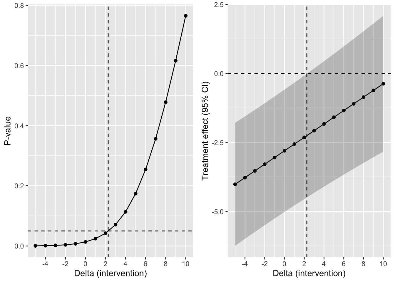
We clearly see that the p-value under MAR reaches a tipping point from 3 onward in the range of delta’s considered.
Delta adjustment for control and intervention arms
Let’s now create a sequence of delta’s for the control group too, and carry out a second tipping point analysis under the MAR assumption.
delta_df2 <- expand.grid(
  delta_control = seq(-3, 8, by = 1),
  delta_intervention = seq(-3, 8, by = 1)
) |>
  as_tibble()
MAR_tipp_df2 <- delta_df2 |>
furrr::future_pmap(perform_tipp_analysis) |>
purrr::reduce(bind_rows)
# Adding back the delta's used for reference
MAR_tipp_df2 <- dplyr::bind_cols(delta_df2, MAR_tipp_df2) |>
mutate(
pval = cut(
pval_7,
c(0, 0.001, 0.01, 0.05, 0.2, 1),
right = FALSE,
labels = c(
"<0.001",
"0.001 - <0.01",
"0.01 - <0.05",
"0.05 - <0.20",
">= 0.20"
)
)
) We can visualize the result of this tipping point analysis using a heatmap. Here, the (0,0) point corresponds to the original result without any delta adjustment (p ~ 0.0125).
MAR_heat <- ggplot(
  MAR_tipp_df2,
  aes(delta_control, delta_intervention, fill = pval)
) +
  geom_raster() +
  scale_fill_manual(
    values = c("darkgreen", "lightgreen", "lightyellow", "orange", "red")
  ) +
  scale_x_continuous(breaks = seq(-5, 10, 1)) +
  scale_y_continuous(breaks = seq(-5, 10, 1)) +
  labs(x = "Delta (control)", y = "Delta (intervention)", fill = "P-value")
MAR_heat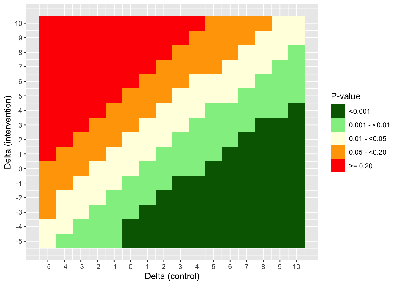
Comparison with rbmi MNAR approaches
Summary of results
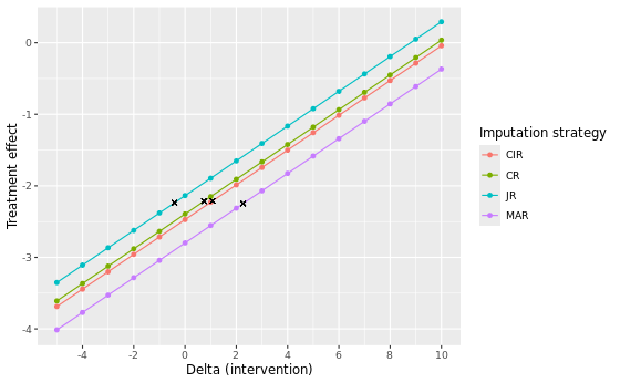
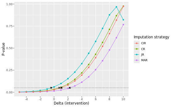
In the table below we present the results of the different imputation strategies with varying number of multiple imputation draws, M = 500 and M = 5000. Note that the results can be slightly different from the results above due to a possible different seed. The estimates show the contrast at visit 7 between DRUG and PLACEBO (DRUG - PLACEBO). Delta adjustments were applied to all imputed missing data in the intervention group only.
| Method | Delta control | Delta intervention at TP | Estimate at TP | 95% CI | P-value | Original estimate | Original p-value |
|---|---|---|---|---|---|---|---|
| MI - MAR (M=500) | 0 | 3 | -2.074 | -4.324 to 0.176 | 0.0709 | -2.798 | 0.0135 |
| MI - MAR (M=5000) | 0 | 3 | -2.100 | -4.354 to 0.154 | 0.0675 | -2.829 | 0.0128 |
| MI - MNAR JR (M=500) | 0 | -1 | -2.380 | -4.595 to -0.165 | 0.0354 | -2.137 | 0.0602 |
| MI - MNAR JR (M=5000) | 0 | -1 | -2.383 | -4.608 to -0.157 | 0.0361 | -2.140 | 0.0611 |
| MI - MNAR CR (M=500) | 0 | 1 | -2.151 | -4.359 to 0.057 | 0.0561 | -2.394 | 0.0326 |
| MI - MNAR CR (M=5000) | 0 | 1 | -2.162 | -4.377 to 0.054 | 0.0558 | -2.405 | 0.0324 |
| MI - MNAR CIR (M=500) | 0 | 2 | -1.986 | -4.211 to 0.239 | 0.0798 | -2.472 | 0.0274 |
| MI - MNAR CIR (M=5000) | 0 | 2 | -1.994 | -4.227 to 0.239 | 0.0796 | -2.480 | 0.0274 |
Of all considered approaches, the MAR approach yields the largest delta adjustment at its tipping point, with a delta intervention of 3 at both M = 500 and M = 5000. This indicates that the MAR assumption is the most robust against slight deviations of its conditions. Notice that for the MNAR JR approach we included, for completeness, tipping point analyses to know when the results switch from non-significant to significant. Correspondingly, two negative delta’s (-1) are found at the tipping point for M = 500 and M = 5000. This is expected, given that the original analyses are non-significant (p ~ 0.0602 and p ~ 0.0611) and a tipping point analysis here aims to find the point at which the analysis turns to be significant, instead of non-significant.
Visual comparison
Flexible delta adjustments
So far, we have only considered simple delta adjustments that add the same value to all imputed missing data. However, you may want to implement more flexible delta adjustments for post-ICE missing data, where the magnitude of the delta varies depending on the distance of the visit from the ICE visit.
To facilitate the creation of such flexible delta adjustments, the delta_template() function has two additional arguments delta and dlag:
delta: specifies the default amount of delta that should be applied to each post-ICE visit (default is NULL)dlag: specifies the scaling coefficient to be applied based upon the visits proximity to the first visit affected by the ICE (default is NULL)
The usage of the delta and dlag arguments is best illustrated with a few examples from the rbmi advanced functionality vignette.
Scaling delta by visit
Assume a setting with 4 visits and the user specified delta = c(5, 6, 7, 8) and dlag = c(1, 2, 3, 4). For a subject for whom the first visit affected by the ICE is visit 2, these values of delta and dlag would imply the following delta offset:
| Visit 1 | Visit 2 | Visit 3 | Visit 4 | |
|---|---|---|---|---|
| Delta | 5 | 6 | 7 | 8 |
| Dlag | 0 | 1 | 2 | 3 |
| Delta * dlag | 0 | 6 | 14 | 24 |
| Cumulative sum | 0 | 6 | 20 | 44 |
That is, the subject would have a delta adjustment of 0 applied to visit 1, 6 for visit 2, 20 for visit 3 and 44 for visit 4.
Assume instead, that the subject’s first visit affected by the ICE was visit 3. Then, the above values of delta and dlag would imply the following delta adjustment:
| Visit 1 | Visit 2 | Visit 3 | Visit 4 | |
|---|---|---|---|---|
| Delta | 5 | 6 | 7 | 8 |
| Dlag | 0 | 0 | 1 | 2 |
| Delta * dlag | 0 | 0 | 7 | 16 |
| Cumulative sum | 0 | 0 | 7 | 23 |
And thus the subject would have a delta adjustment of 0 applied to visits 1 and 2, 7 for visit 3 and 23 for visit 4.
Another way of using these arguments is to set delta to the difference in time between visits and dlag to be the amount of delta per unit of time. For example, let’s say that visits occur on weeks 1, 5, 6 and 9 and that we want a delta of 3 to be applied for each week after an ICE. For simplicity, we assume that the ICE occurs immediately after the subject’s last visit which is not affected by the ICE. This could be achieved by setting delta = c(1, 4, 1, 3), i.e. the difference in weeks between each visit, and dlag = c(3, 3, 3, 3).
Assume a subject’s first visit affected by the ICE was visit 2, then these values of delta and dlag would imply the following delta adjustment:
| Visit 1 | Visit 2 | Visit 3 | Visit 4 | |
|---|---|---|---|---|
| Delta | 1 | 4 | 1 | 3 |
| Dlag | 0 | 3 | 3 | 3 |
| Delta * dlag | 0 | 12 | 3 | 9 |
| Cumulative sum | 0 | 12 | 15 | 24 |
Let’s now consider the antidepressant data again. Suppose we apply a delta adjustment of 2 for each week following an ICE in the intervention group only. For example, if the ICE took place immediately after visit 4, then the cumulative delta applied to a missing value from visit 5 would be 2, from visit 6 would be 4, and from visit 7 would be 6.
To program this, we first use the delta and dlag arguments of delta_template().
dat_delta <- rbmi::delta_template(
  imputeObj,
  delta = c(2, 2, 2, 2),
  dlag = c(1, 1, 1, 1)
)

dat_delta |>
  dplyr::filter(PATIENT %in% c("1513", "1514")) |>
  head(8) |>
gt()| PATIENT | VISIT | THERAPY | is_mar | is_missing | is_post_ice | strategy | delta |
|---|---|---|---|---|---|---|---|
| 1513 | 4 | DRUG | TRUE | FALSE | FALSE | NA | 0 |
| 1513 | 5 | DRUG | TRUE | TRUE | TRUE | MAR | 2 |
| 1513 | 6 | DRUG | TRUE | TRUE | TRUE | MAR | 4 |
| 1513 | 7 | DRUG | TRUE | TRUE | TRUE | MAR | 6 |
| 1514 | 4 | PLACEBO | TRUE | FALSE | FALSE | NA | 0 |
| 1514 | 5 | PLACEBO | TRUE | TRUE | TRUE | MAR | 2 |
| 1514 | 6 | PLACEBO | TRUE | TRUE | TRUE | MAR | 4 |
| 1514 | 7 | PLACEBO | TRUE | TRUE | TRUE | MAR | 6 |
Then, we use some metadata variables provided by delta_template() to manually reset the delta values for the control group back to 0.
dat_delta <- dat_delta |>
  mutate(delta = if_else(THERAPY == "PLACEBO", 0, delta))

dat_delta |>
  dplyr::filter(PATIENT %in% c("1513", "1514")) |>
  head(8) |>
gt()| PATIENT | VISIT | THERAPY | is_mar | is_missing | is_post_ice | strategy | delta |
|---|---|---|---|---|---|---|---|
| 1513 | 4 | DRUG | TRUE | FALSE | FALSE | NA | 0 |
| 1513 | 5 | DRUG | TRUE | TRUE | TRUE | MAR | 2 |
| 1513 | 6 | DRUG | TRUE | TRUE | TRUE | MAR | 4 |
| 1513 | 7 | DRUG | TRUE | TRUE | TRUE | MAR | 6 |
| 1514 | 4 | PLACEBO | TRUE | FALSE | FALSE | NA | 0 |
| 1514 | 5 | PLACEBO | TRUE | TRUE | TRUE | MAR | 0 |
| 1514 | 6 | PLACEBO | TRUE | TRUE | TRUE | MAR | 0 |
| 1514 | 7 | PLACEBO | TRUE | TRUE | TRUE | MAR | 0 |
And lastly we use dat_delta to apply the desired delta offset to our analysis model under the delta argument of the analyse() function.
anaObj <- rbmi::analyse(
  imputations = imputeObj,
  fun = ancova,
  delta = dat_delta,
  vars = vars_analyse
)

poolObj <- rbmi::pool(anaObj)
Fixed delta
You may also add a simple, fixed delta using the delta and dlag arguments. To do this, delta should be specified as a vector of length equal to the amount of visits, e.g. c(5, 5, 5, 5), while dlag should be c(1, 0, 0, 0). This ensures a delta of 5 is added to each imputed missing value following an ICE, which we here assume to occur at the visit 2:
| Visit 1 | Visit 2 | Visit 3 | Visit 4 | |
|---|---|---|---|---|
| Delta | 5 | 5 | 5 | 5 |
| Dlag | 0 | 1 | 0 | 0 |
| Delta * dlag | 0 | 0 | 0 | 0 |
| Cumulative sum | 0 | 5 | 5 | 5 |
Adding a fixed delta in this way seems similar to what we explained in the simple delta adjustments section above, but there are some crucial differences. Remember the first case where we added delta = 5 to all imputed is_missing values:
# 1) mutate delta = is_missing * 5
dat_delta_5_v1 <- delta_template(imputations = imputeObj) |>
  mutate(delta = is_missing * 5)
And remember the second case where we added delta = 5 to all imputed is_missing and is_post_ice values:
# 2) mutate delta = is_missing * is_post_ice * 5
dat_delta_5_v2 <- delta_template(imputations = imputeObj) |>
  mutate(delta = is_missing * is_post_ice * 5)
Similarly, we now set delta = c(5, 5, 5, 5) and dlag = c(1, 0, 0, 0):
# 3) delta = c(5, 5, 5, 5), dlag = c(1, 0, 0, 0)
dat_delta_5_v3 <- delta_template(
  imputeObj,
  delta = c(5, 5, 5, 5),
  dlag = c(1, 0, 0, 0)
)
The difference between these three approaches lies in how they treat intermittent missing values that do not correspond to study drug discontinuation due to an ICE.
If we consider patient 3618 again, we see that its intermittent missing value at visit 5 has delta = 5 added in the first approach (using is_missing * 5), while this missing value is not considered at all to receive a delta adjustment in the second or third approach (using is_missing * is_post_ice * 5, or delta = c(5, 5, 5, 5) and dlag = c(1, 0, 0, 0)). Thus by default, the delta and dlag arguments of delta_template() (third approach) only add delta adjustments to post-ICE missing values.
# imputed dataset without delta adjustment
gt(MI_10 |> dplyr::filter(PATIENT == "3618"))| PATIENT | GENDER | THERAPY | RELDAYS | VISIT | BASVAL | HAMDTL17 | CHANGE | PATIENT2 |
|---|---|---|---|---|---|---|---|---|
| 3618 | M | DRUG | 8 | 4 | 8 | 15 | 7.000000 | new_pt_99 |
| 3618 | M | DRUG | NA | 5 | 8 | NA | 1.135327 | new_pt_99 |
| 3618 | M | DRUG | 28 | 6 | 8 | 14 | 6.000000 | new_pt_99 |
| 3618 | M | DRUG | 42 | 7 | 8 | 10 | 2.000000 | new_pt_99 |
# 1) mutate delta = is_missing * 5
rbmi:::apply_delta(
  MI_10,
  delta = dat_delta_5_v1,
  group = c("PATIENT", "VISIT", "THERAPY"),
  outcome = "CHANGE"
) |>
  dplyr::filter(PATIENT == 3618) |>
gt()| PATIENT | GENDER | THERAPY | RELDAYS | VISIT | BASVAL | HAMDTL17 | CHANGE | PATIENT2 |
|---|---|---|---|---|---|---|---|---|
| 3618 | M | DRUG | 8 | 4 | 8 | 15 | 7.000000 | new_pt_99 |
| 3618 | M | DRUG | NA | 5 | 8 | NA | 6.135327 | new_pt_99 |
| 3618 | M | DRUG | 28 | 6 | 8 | 14 | 6.000000 | new_pt_99 |
| 3618 | M | DRUG | 42 | 7 | 8 | 10 | 2.000000 | new_pt_99 |
# 2) mutate delta = is_missing * is_post_ice * 5
rbmi:::apply_delta(
  MI_10,
  delta = dat_delta_5_v2,
  group = c("PATIENT", "VISIT", "THERAPY"),
  outcome = "CHANGE"
) |>
  dplyr::filter(PATIENT == 3618) |>
gt()| PATIENT | GENDER | THERAPY | RELDAYS | VISIT | BASVAL | HAMDTL17 | CHANGE | PATIENT2 |
|---|---|---|---|---|---|---|---|---|
| 3618 | M | DRUG | 8 | 4 | 8 | 15 | 7.000000 | new_pt_99 |
| 3618 | M | DRUG | NA | 5 | 8 | NA | 1.135327 | new_pt_99 |
| 3618 | M | DRUG | 28 | 6 | 8 | 14 | 6.000000 | new_pt_99 |
| 3618 | M | DRUG | 42 | 7 | 8 | 10 | 2.000000 | new_pt_99 |
# 3) delta = c(5, 5, 5, 5), dlag = c(1, 0, 0, 0)
rbmi:::apply_delta(
  MI_10,
  delta = dat_delta_5_v3,
  group = c("PATIENT", "VISIT", "THERAPY"),
  outcome = "CHANGE"
) |>
  dplyr::filter(PATIENT == 3618) |>
gt()| PATIENT | GENDER | THERAPY | RELDAYS | VISIT | BASVAL | HAMDTL17 | CHANGE | PATIENT2 |
|---|---|---|---|---|---|---|---|---|
| 3618 | M | DRUG | 8 | 4 | 8 | 15 | 7.000000 | new_pt_99 |
| 3618 | M | DRUG | NA | 5 | 8 | NA | 1.135327 | new_pt_99 |
| 3618 | M | DRUG | 28 | 6 | 8 | 14 | 6.000000 | new_pt_99 |
| 3618 | M | DRUG | 42 | 7 | 8 | 10 | 2.000000 | new_pt_99 |
One should be aware of this discrepancy when using the rbmi package for delta adjustments. For all tipping point analyses performed under MAR and MNAR in this tutorial, we adopted the first approach and applied delta adjustments to all imputed missing data. In contrast, we note that the five macros in SAS uses the second delta and dlag approach as discussed here, i.e. it does not apply delta adjustments to intermittent missing values. This could have important implications for datasets with high proportions of intermittent missing values, as it could alter the results of the tipping point analysis substantially.
References
Cro et al. 2020. Sensitivity analysis for clinical trials with missing continuous outcome data using controlled multiple imputation: A practical guide. Statistics in Medicine. 2020;39(21):2815-2842.
Gower-Page et al. 2022. rbmi: A R package for standard and reference-based multiple imputation methods. Journal of Open Source Software 7(74):4251.
rbmi: Reference-Based Multiple Imputation
Roger 2022. Other statistical software for continuous longitudinal endpoints: SAS macros for multiple imputation. Addressing intercurrent events: Treatment policy and hypothetical strategies. Joint EFSPI and BBS virtual event.
Roger 2017. Fitting reference-based models for missing data to longitudinal repeated-measures Normal data. User guide five macros.
NoteSession info
─ Session info ───────────────────────────────────────────────────────────────
 setting  value
 version  R version 4.5.2 (2025-10-31)
 os       Ubuntu 24.04.3 LTS
 system   x86_64, linux-gnu
 ui       X11
 language (EN)
 collate  en_US.UTF-8
 ctype    en_US.UTF-8
 tz       Europe/London
 date     2026-03-17
 pandoc   3.6.3 @ /home/michael/.positron-server/bin/f3aae65e0a1a11d39226cd884520f49301daef82/quarto/bin/tools/x86_64/ (via rmarkdown)

─ Packages ───────────────────────────────────────────────────────────────────
 ! package      * version  date (UTC) lib source
 P assertthat     0.2.1    2019-03-21 [?] RSPM (R 4.5.0)
 P backports      1.5.0    2024-05-23 [?] RSPM (R 4.5.0)
   boot           1.3-32   2025-08-29 [2] CRAN (R 4.5.2)
 P broom          1.0.12   2026-01-27 [?] RSPM (R 4.5.0)
 P callr          3.7.6    2024-03-25 [?] RSPM (R 4.5.0)
 P checkmate      2.3.4    2026-02-03 [?] RSPM (R 4.5.0)
 P cli            3.6.5    2025-04-23 [?] RSPM (R 4.5.0)
   codetools      0.2-20   2024-03-31 [2] CRAN (R 4.5.2)
 P curl           7.0.0    2025-08-19 [?] RSPM (R 4.5.0)
 P digest         0.6.39   2025-11-19 [?] RSPM (R 4.5.0)
 P dplyr        * 1.2.0    2026-02-03 [?] RSPM (R 4.5.0)
 P emmeans      * 2.0.1    2025-12-16 [?] RSPM (R 4.5.0)
 P estimability   1.5.1    2024-05-12 [?] RSPM (R 4.5.0)
 P evaluate       1.0.5    2025-08-27 [?] RSPM (R 4.5.0)
 P farver         2.1.2    2024-05-13 [?] RSPM (R 4.5.0)
 P fastmap        1.2.0    2024-05-15 [?] RSPM (R 4.5.0)
 P forcats        1.0.1    2025-09-25 [?] RSPM (R 4.5.0)
 P foreach        1.5.2    2022-02-02 [?] RSPM (R 4.5.0)
 P fs             1.6.6    2025-04-12 [?] RSPM (R 4.5.0)
 P furrr        * 0.3.1    2022-08-15 [?] RSPM (R 4.5.0)
 P future       * 1.69.0   2026-01-16 [?] RSPM (R 4.5.0)
 P generics       0.1.4    2025-05-09 [?] RSPM (R 4.5.0)
 P ggplot2      * 4.0.2    2026-02-03 [?] RSPM (R 4.5.0)
 P glmnet         4.1-10   2025-07-17 [?] RSPM (R 4.5.0)
 P globals        0.19.0   2026-02-02 [?] RSPM (R 4.5.0)
 P glue           1.8.0    2024-09-30 [?] RSPM (R 4.5.0)
 P gridExtra    * 2.3      2017-09-09 [?] RSPM (R 4.5.0)
 P gt           * 1.3.0    2026-01-22 [?] RSPM (R 4.5.0)
 P gtable         0.3.6    2024-10-25 [?] RSPM (R 4.5.0)
 P haven          2.5.5    2025-05-30 [?] RSPM (R 4.5.0)
 P hms            1.1.4    2025-10-17 [?] RSPM (R 4.5.0)
 P htmltools      0.5.9    2025-12-04 [?] RSPM (R 4.5.0)
 P htmlwidgets    1.6.4    2023-12-06 [?] RSPM (R 4.5.0)
 P inline         0.3.21   2025-01-09 [?] RSPM (R 4.5.0)
 P iterators      1.0.14   2022-02-05 [?] RSPM (R 4.5.0)
 P jinjar         0.3.2    2025-03-13 [?] RSPM (R 4.5.0)
 P jomo           2.7-6    2023-04-15 [?] RSPM (R 4.5.0)
 P jsonlite       2.0.0    2025-03-27 [?] RSPM (R 4.5.0)
 P knitr          1.51     2025-12-20 [?] RSPM (R 4.5.0)
 P labeling       0.4.3    2023-08-29 [?] RSPM (R 4.5.0)
 P labelled     * 2.16.0   2025-10-22 [?] RSPM (R 4.5.0)
   lattice        0.22-7   2025-04-02 [2] CRAN (R 4.5.2)
 P lifecycle      1.0.5    2026-01-08 [?] RSPM (R 4.5.0)
 P listenv        0.10.0   2025-11-02 [?] RSPM (R 4.5.0)
 P lme4           1.1-38   2025-12-02 [?] RSPM (R 4.5.0)
 P loo            2.9.0    2025-12-23 [?] RSPM (R 4.5.0)
 P magrittr       2.0.4    2025-09-12 [?] RSPM (R 4.5.0)
   MASS           7.3-65   2025-02-28 [2] CRAN (R 4.5.2)
   Matrix         1.7-4    2025-08-28 [2] CRAN (R 4.5.2)
 P matrixStats    1.5.0    2025-01-07 [?] RSPM (R 4.5.0)
 P mice         * 3.19.0   2025-12-10 [?] RSPM (R 4.5.0)
 P minqa          1.2.8    2024-08-17 [?] RSPM (R 4.5.0)
 P mitml          0.4-5    2023-03-08 [?] RSPM (R 4.5.0)
 P mmrm         * 0.3.17   2026-01-08 [?] RSPM (R 4.5.0)
 P multcomp       1.4-29   2025-10-20 [?] RSPM (R 4.5.0)
 P mvtnorm        1.3-3    2025-01-10 [?] RSPM (R 4.5.0)
   nlme           3.1-168  2025-03-31 [2] CRAN (R 4.5.2)
 P nloptr         2.2.1    2025-03-17 [?] RSPM (R 4.5.0)
   nnet           7.3-20   2025-01-01 [2] CRAN (R 4.5.2)
 P otel           0.2.0    2025-08-29 [?] RSPM (R 4.5.0)
 P pan            1.9      2023-12-07 [?] RSPM (R 4.5.0)
 P parallelly   * 1.46.1   2026-01-08 [?] RSPM (R 4.5.0)
 P pillar         1.11.1   2025-09-17 [?] RSPM (R 4.5.0)
 P pkgbuild       1.4.8    2025-05-26 [?] RSPM (R 4.5.0)
 P pkgconfig      2.0.3    2019-09-22 [?] RSPM (R 4.5.0)
 P processx       3.8.6    2025-02-21 [?] RSPM (R 4.5.0)
 P ps             1.9.1    2025-04-12 [?] RSPM (R 4.5.0)
 P purrr        * 1.2.1    2026-01-09 [?] RSPM (R 4.5.0)
 P QuickJSR       1.9.0    2026-01-25 [?] RSPM (R 4.5.0)
 P R6             2.6.1    2025-02-15 [?] RSPM (R 4.5.0)
 P rbibutils      2.4.1    2026-01-21 [?] RSPM (R 4.5.0)
 P rbmi         * 1.6.0    2026-01-23 [?] RSPM (R 4.5.0)
 P RColorBrewer   1.1-3    2022-04-03 [?] RSPM (R 4.5.0)
 P Rcpp           1.1.1    2026-01-10 [?] RSPM (R 4.5.0)
 P RcppParallel   5.1.11-1 2025-08-27 [?] RSPM (R 4.5.0)
 P Rdpack         2.6.6    2026-02-08 [?] RSPM (R 4.5.0)
 P reformulas     0.4.4    2026-02-02 [?] RSPM (R 4.5.0)
   renv           1.0.10   2024-10-05 [1] RSPM (R 4.5.2)
 P rlang          1.1.7    2026-01-09 [?] RSPM (R 4.5.0)
 P rmarkdown      2.30     2025-09-28 [?] RSPM (R 4.5.0)
   rpart          4.1.24   2025-01-07 [2] CRAN (R 4.5.2)
 P rstan        * 2.32.7   2025-03-10 [?] RSPM (R 4.5.0)
 P S7             0.2.1    2025-11-14 [?] RSPM (R 4.5.0)
 P sandwich       3.1-1    2024-09-15 [?] RSPM (R 4.5.0)
 P sass           0.4.10   2025-04-11 [?] RSPM (R 4.5.0)
 P scales         1.4.0    2025-04-24 [?] RSPM (R 4.5.0)
 P sessioninfo    1.2.2    2021-12-06 [?] RSPM (R 4.5.0)
 P shape          1.4.6.1  2024-02-23 [?] RSPM (R 4.5.0)
 P StanHeaders  * 2.32.10  2024-07-15 [?] RSPM (R 4.5.0)
 P stringi        1.8.7    2025-03-27 [?] RSPM (R 4.5.0)
 P stringr        1.6.0    2025-11-04 [?] RSPM (R 4.5.0)
   survival       3.8-3    2024-12-17 [2] CRAN (R 4.5.2)
 P TH.data        1.1-5    2025-11-17 [?] RSPM (R 4.5.0)
 P tibble         3.3.1    2026-01-11 [?] RSPM (R 4.5.0)
 P tidyr        * 1.3.2    2025-12-19 [?] RSPM (R 4.5.0)
 P tidyselect     1.2.1    2024-03-11 [?] RSPM (R 4.5.0)
 P TMB            1.9.19   2025-12-15 [?] RSPM (R 4.5.0)
 P utf8           1.2.6    2025-06-08 [?] RSPM (R 4.5.0)
 P V8             8.0.1    2025-10-10 [?] RSPM (R 4.5.0)
 P vctrs          0.7.1    2026-01-23 [?] RSPM (R 4.5.0)
 P withr          3.0.2    2024-10-28 [?] RSPM (R 4.5.0)
 P xfun           0.56     2026-01-18 [?] RSPM (R 4.5.0)
 P xml2           1.5.2    2026-01-17 [?] RSPM (R 4.5.0)
 P xtable         1.8-4    2019-04-21 [?] RSPM (R 4.5.0)
 P yaml           2.3.12   2025-12-10 [?] RSPM (R 4.5.0)
 P zoo            1.8-15   2025-12-15 [?] RSPM (R 4.5.0)

 [1] /home/michael/source/personal/CAMIS/renv/library/linux-ubuntu-noble/R-4.5/x86_64-pc-linux-gnu
 [2] /opt/R/4.5.2/lib/R/library

 P ── Loaded and on-disk path mismatch.

──────────────────────────────────────────────────────────────────────────────